Part 1: Geostrophic balance
Andrew Delman, updated 2023-12-22.
Objectives
To use ECCO state estimate output to illustrate the concept of geostrophic balance; where it does and doesn’t explain oceanic flows well.
By the end of the tutorial, you will be able to:
Download ECCO fields and query their attributes using
xarray
Plot ECCO fields on a single tile
Carry out spatial differencing and interpolation on the ECCO native model grid
Compare the two sides of the geostrophic balance equations
Compute geostrophic velocities
Apply masks in 2-D spatial plots
Use the
ecco_v4_py
package to plot global maps of ECCO fieldsUse a statistical measure (normalized difference) to assess the latitude and depth dependence of geostrophic balance
Introduction
Conservation of momentum
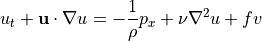
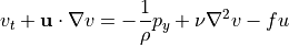
Geostrophic balance originates from the conservation of momentum, as expressed by the momentum equation:
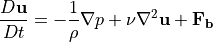
following roughly the notation used in Kundu and Cohen (2008) and Vallis (2006). This equation is a simplification of the Navier-Stokes equation for an incompressible fluid. The material derivative 
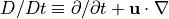
is the derivative in time following a fluid parcel. The symbol indicates the kinematic viscosity, and represents body forces (real or apparent) exerted on the fluid.
The equation above applies to any incompressible fluid, even the water in a fish tank or swimming pool. However, the body forces are dependent upon the environment of the fluid and the scales being considered. In a physical oceanography context, three forces that are typically very important are (a) gravity, (b) the Coriolis force from rotation of the earth, and (c) friction from surface winds or topography. So the equation above can be rewritten as
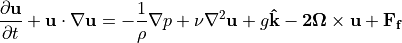
Of those last three terms: 1. Gravity effectively only applies to vertical momentum, and can be neglected in the horizontal momentum equations 1. The Coriolis force can be approximated by its vertical component,
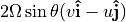
 where is the rotation rate of Earth in radians and is latitude 1. Friction from wind and topography is negligible in the ocean interior.
To simplify, is defined as . So using subscript notation for derivatives ( is the derivative of with respect to ) the two horizontal components of momentum conservation are:
Geostrophic balance
The two horizontal momentum equations still have a number of terms, but in the global oceans most of the flow is explained by a balance between just two terms. In steady state (or for very slowly-varying ocean features) the time derivatives , are negligible, and at the large scales of major ocean currents viscosity is relatively small as well (inviscid approximation). This leaves three terms. The 2nd term on the left-hand side is usually negligible at large scales as well (we’ll return to this later), so large-scale ocean flows generally follow geostrophic balance:
(cf. Vallis ch. 2.8, Kundu and Cohen ch. 14.5, Gill ch. 7.6)
If you’ve looked at weather maps that show the clockwise or counter-clockwise flow of winds around areas of high or low pressure, you’ve encountered geostrophic balance in the atmosphere. But what does it look like in the ocean? You’re about to see it in action…using output from the ECCO state estimate.
Download the ECCO output
If you haven’t been through the Using Python to Download ECCO Datasets tutorial yet, I recommend going through it before proceeding further with this tutorial. If you’ve done that tutorial, you can save the ecco_download.py file on your local machine and use it to get the output we need to assess geostrophic balance.
What fields will we need? Look at the geostrophic balance equations. On the left-hand side, the Coriolis parameter is a function of latitude which we can compute, so we only need to download horizontal velocities and . On the right-hand side we need density and pressure , as well as the grid parameters that allow us to compute spatial derivatives.
Here are the lists of variables contained in ECCOv4r4 datasets on PO.DAAC:
ECCO v4r4 llc90 Grid Dataset Variables - Monthly Means
ECCO v4r4 llc90 Grid Dataset Variables - Daily Means
ECCO v4r4 llc90 Grid Dataset Variables - Daily Snapshots
ECCO v4r4 0.5-Deg Interp Grid Dataset Variables - Monthly Means
ECCO v4r4 0.5-Deg Interp Grid Dataset Variables - Daily Means
ECCO v4r4 Time Series and Grid Parameters
Let’s have a look at the llc90 grid monthly means variable list. A text search for “velocity” shows us that UVEL and VVEL are the horizontal velocity variables we need. Importantly, we need to know the ShortName of the datasets containing these variables, which is ECCO_L4_OCEAN_VEL_LLC0090GRID_MONTHLY_V4R4.
Searching for “density” and we get RHOAnoma (in-situ seawater density anomaly), and “pressure” gives us PHIHYD and PHIHYDcR (ocean hydrostatic pressure anomaly)–in this analysis we specifically need to use PHIHYDcR, the pressure anomaly at constant depth. These fields are all found in datasets with ShortName ECCO_L4_DENS_STRAT_PRESS_LLC0090GRID_MONTHLY_V4R4.
Now that the datasets we need have been identified, let’s download them for the month of January 2000.
Tip: do you find yourself having to say “PO.DAAC”, and wondering if you have to spell out all of those letters? Please don’t…spare yourself! It’s pronounced Poh-dack, and rhymes with “low stack”, as in the amount of homework you can only hope for as a 1st year PO grad student. :-o
[1]:
# # only need this if ecco_download.py is in a different directory than the tutorial notebook
# import sys
# sys.path.append('/home/user/some_other_directory')
# load module into workspace
from ecco_download import ecco_podaac_download
# query to see the syntax needed for the download function, using help(), or put ? after the function name
help(ecco_podaac_download)
Help on function ecco_podaac_download in module ecco_download:
ecco_podaac_download(ShortName, StartDate, EndDate, download_root_dir=None, n_workers=6, force_redownload=False)
This routine downloads ECCO datasets from PO.DAAC. It is adapted from the Jupyter notebooks
created by Jack McNelis and Ian Fenty (https://github.com/ECCO-GROUP/ECCO-ACCESS/blob/master/PODAAC/Downloading_ECCO_datasets_from_PODAAC/README.md)
and modified by Andrew Delman (https://ecco-v4-python-tutorial.readthedocs.io).
Parameters
----------
ShortName: str, the ShortName that identifies the dataset on PO.DAAC.
StartDate,EndDate: str, in 'YYYY', 'YYYY-MM', or 'YYYY-MM-DD' format,
define date range [StartDate,EndDate] for download.
EndDate is included in the time range (unlike typical Python ranges).
ECCOv4r4 date range is '1992-01-01' to '2017-12-31'.
For 'SNAPSHOT' datasets, an additional day is added to EndDate to enable closed budgets
within the specified date range.
n_workers: int, number of workers to use in concurrent downloads.
force_redownload: bool, if True, existing files will be redownloaded and replaced;
if False, existing files will not be replaced.
[2]:
# download file (granule) containing Jan 2000 velocities,
# to default path ~/Downloads/ECCO_V4r4_PODAAC/
vel_monthly_shortname = "ECCO_L4_OCEAN_VEL_LLC0090GRID_MONTHLY_V4R4"
ecco_podaac_download(ShortName=vel_monthly_shortname,\
StartDate="2000-01-01",EndDate="2000-01-31",download_root_dir=None,\
n_workers=6,force_redownload=False)
created download directory C:\Users\adelman\Downloads\ECCO_V4r4_PODAAC\ECCO_L4_OCEAN_VEL_LLC0090GRID_MONTHLY_V4R4
Total number of matching granules: 1
DL Progress: 100%|###########################| 1/1 [00:06<00:00, 6.01s/it]
=====================================
total downloaded: 30.6 Mb
avg download speed: 5.07 Mb/s
Time spent = 6.032305955886841 seconds
[3]:
# download file (granule) containing Jan 2000 density/pressure anomalies,
# to default path ~/Downloads/ECCO_V4r4_PODAAC/
denspress_monthly_shortname = "ECCO_L4_DENS_STRAT_PRESS_LLC0090GRID_MONTHLY_V4R4"
ecco_podaac_download(ShortName=denspress_monthly_shortname,\
StartDate="2000-01-01",EndDate="2000-01-31",download_root_dir=None,\
n_workers=6,force_redownload=False)
created download directory C:\Users\adelman\Downloads\ECCO_V4r4_PODAAC\ECCO_L4_DENS_STRAT_PRESS_LLC0090GRID_MONTHLY_V4R4
Total number of matching granules: 1
DL Progress: 100%|###########################| 1/1 [00:07<00:00, 7.11s/it]
=====================================
total downloaded: 30.98 Mb
avg download speed: 4.36 Mb/s
Time spent = 7.113083362579346 seconds
Notice that the StartDate for each of the downloads was set to the 2nd of the month (2000-01-02) not the 1st. If it is set to the 1st, then the file for Dec 1999 will also be downloaded (which ends on 2000-01-01).
Once you have downloaded the monthly files for velocities and density/pressure, let’s also download daily files for each (2000-01-01). Consulting the “Daily Means” list of variables, the ShortNames of the datasets needed are very similar; MONTHLY is just replaced with DAILY.
[4]:
# download file (granule) containing 01 Jan 2000 velocities,
# to default path ~/Downloads/ECCO_V4r4_PODAAC/
vel_daily_shortname = "ECCO_L4_OCEAN_VEL_LLC0090GRID_DAILY_V4R4"
ecco_podaac_download(ShortName=vel_daily_shortname,\
StartDate="2000-01-01",EndDate="2000-01-01",download_root_dir=None,\
n_workers=6,force_redownload=False)
# download file (granule) containing 01 Jan 2000 density/pressure anomalies,
# to default path ~/Downloads/ECCO_V4r4_PODAAC/
denspress_daily_shortname = "ECCO_L4_DENS_STRAT_PRESS_LLC0090GRID_DAILY_V4R4"
ecco_podaac_download(ShortName=denspress_daily_shortname,\
StartDate="2000-01-01",EndDate="2000-01-01",download_root_dir=None,\
n_workers=6,force_redownload=False)
created download directory C:\Users\adelman\Downloads\ECCO_V4r4_PODAAC\ECCO_L4_OCEAN_VEL_LLC0090GRID_DAILY_V4R4
Total number of matching granules: 1
DL Progress: 100%|###########################| 1/1 [00:06<00:00, 6.58s/it]
=====================================
total downloaded: 30.68 Mb
avg download speed: 4.65 Mb/s
Time spent = 6.5920562744140625 seconds
created download directory C:\Users\adelman\Downloads\ECCO_V4r4_PODAAC\ECCO_L4_DENS_STRAT_PRESS_LLC0090GRID_DAILY_V4R4
Total number of matching granules: 1
DL Progress: 100%|###########################| 1/1 [00:04<00:00, 4.97s/it]
=====================================
total downloaded: 31.2 Mb
avg download speed: 6.27 Mb/s
Time spent = 4.976189613342285 seconds
Last but not least, we will need certain parameters from the model grid in order to compute gradients (derivatives with respect to and ). These are in a dataset with ShortName ECCO_L4_GEOMETRY_LLC0090GRID_V4R4; they have no time dimension but setting StartDate
and EndDate
for any date between 1992-01-01 and 2018-01-01 should download it.
[5]:
grid_params_shortname = "ECCO_L4_GEOMETRY_LLC0090GRID_V4R4"
ecco_podaac_download(ShortName=grid_params_shortname,\
StartDate="2000-01-01",EndDate="2000-01-01",download_root_dir=None,\
n_workers=6,force_redownload=False)
created download directory C:\Users\adelman\Downloads\ECCO_V4r4_PODAAC\ECCO_L4_GEOMETRY_LLC0090GRID_V4R4
Total number of matching granules: 1
DL Progress: 100%|###########################| 1/1 [00:03<00:00, 3.74s/it]
=====================================
total downloaded: 8.57 Mb
avg download speed: 2.29 Mb/s
Time spent = 3.7480597496032715 seconds
Now check the directory where the ECCO output was downloaded to, this will be under ~/Downloads/ECCO_V4r4_PODAAC/ unless you changed the path under the download_root_dir
option. There should be (at least) 5 subfolders corresponding to 2 datasets each of monthly and daily means, as well as a folder for the grid parameters. The monthly mean folders contain 1 file each for Jan 2000, the daily mean folders contain 2 files each (1999-12-31 and 2000-01-01).
Open/view ECCO files
View and plot density/pressure anomalies on a single “tile”
Now let’s load one of our datasets and create a couple plots. First we’ll load some Python packages that will help us read and plot the data, then we’ll load the monthly density/stratification/pressure dataset into our workspace.
Tip: If you have any errors involving reading the netCDF file in the code below, try installing the
netCDF4
orh5netcdf
packages, using pip install {pkgname} or conda install -c conda-forge {pkgname}.
[6]:
import numpy as np
import xarray as xr
import xmitgcm
import xgcm
import glob
from os.path import expanduser,join
import sys
user_home_dir = expanduser('~')
sys.path.append(join(user_home_dir,'ECCOv4-py'))
import ecco_v4_py as ecco
import matplotlib.pyplot as plt
# locate files to load
download_root_dir = join(user_home_dir,'Downloads','ECCO_V4r4_PODAAC')
download_dir = join(download_root_dir,denspress_monthly_shortname)
curr_denspress_files = list(glob.glob(join(download_dir,'*nc')))
print(f'number of files to load: {len(curr_denspress_files)}')
# load file into workspace
# (in this case only 1 file, but this function can load multiple netCDF files with compatible dimensions)
ds_denspress_mo = xr.open_mfdataset(curr_denspress_files, parallel=True, data_vars='minimal',\
coords='minimal', compat='override')
number of files to load: 1
We have just loaded the contents of the netCDF file into the workspace using the package xarray
. We can look at a summary of the contents of this xarray DataSet:
[7]:
ds_denspress_mo
[7]:
<xarray.Dataset> Dimensions: (i: 90, i_g: 90, j: 90, j_g: 90, k: 50, k_u: 50, k_l: 50, k_p1: 51, tile: 13, time: 1, nv: 2, nb: 4) Coordinates: (12/22) * i (i) int32 0 1 2 3 4 5 6 7 8 9 ... 80 81 82 83 84 85 86 87 88 89 * i_g (i_g) int32 0 1 2 3 4 5 6 7 8 9 ... 80 81 82 83 84 85 86 87 88 89 * j (j) int32 0 1 2 3 4 5 6 7 8 9 ... 80 81 82 83 84 85 86 87 88 89 * j_g (j_g) int32 0 1 2 3 4 5 6 7 8 9 ... 80 81 82 83 84 85 86 87 88 89 * k (k) int32 0 1 2 3 4 5 6 7 8 9 ... 40 41 42 43 44 45 46 47 48 49 * k_u (k_u) int32 0 1 2 3 4 5 6 7 8 9 ... 40 41 42 43 44 45 46 47 48 49 ... ... Zu (k_u) float32 dask.array<chunksize=(50,), meta=np.ndarray> Zl (k_l) float32 dask.array<chunksize=(50,), meta=np.ndarray> time_bnds (time, nv) datetime64[ns] dask.array<chunksize=(1, 2), meta=np.ndarray> XC_bnds (tile, j, i, nb) float32 dask.array<chunksize=(13, 90, 90, 4), meta=np.ndarray> YC_bnds (tile, j, i, nb) float32 dask.array<chunksize=(13, 90, 90, 4), meta=np.ndarray> Z_bnds (k, nv) float32 dask.array<chunksize=(50, 2), meta=np.ndarray> Dimensions without coordinates: nv, nb Data variables: RHOAnoma (time, k, tile, j, i) float32 dask.array<chunksize=(1, 50, 13, 90, 90), meta=np.ndarray> DRHODR (time, k_l, tile, j, i) float32 dask.array<chunksize=(1, 50, 13, 90, 90), meta=np.ndarray> PHIHYD (time, k, tile, j, i) float32 dask.array<chunksize=(1, 50, 13, 90, 90), meta=np.ndarray> PHIHYDcR (time, k, tile, j, i) float32 dask.array<chunksize=(1, 50, 13, 90, 90), meta=np.ndarray> Attributes: (12/62) acknowledgement: This research was carried out by the Jet... author: Ian Fenty and Ou Wang cdm_data_type: Grid comment: Fields provided on the curvilinear lat-l... Conventions: CF-1.8, ACDD-1.3 coordinates_comment: Note: the global 'coordinates' attribute... ... ... time_coverage_duration: P1M time_coverage_end: 2000-02-01T00:00:00 time_coverage_resolution: P1M time_coverage_start: 2000-01-01T00:00:00 title: ECCO Ocean Density, Stratification, and ... uuid: 166a1992-4182-11eb-82f9-0cc47a3f43f9
- i: 90
- i_g: 90
- j: 90
- j_g: 90
- k: 50
- k_u: 50
- k_l: 50
- k_p1: 51
- tile: 13
- time: 1
- nv: 2
- nb: 4
- i(i)int320 1 2 3 4 5 6 ... 84 85 86 87 88 89
- axis :
- X
- long_name :
- grid index in x for variables at tracer and 'v' locations
- swap_dim :
- XC
- comment :
- In the Arakawa C-grid system, tracer (e.g., THETA) and 'v' variables (e.g., VVEL) have the same x coordinate on the model grid.
- coverage_content_type :
- coordinate
array([ 0, 1, 2, 3, 4, 5, 6, 7, 8, 9, 10, 11, 12, 13, 14, 15, 16, 17, 18, 19, 20, 21, 22, 23, 24, 25, 26, 27, 28, 29, 30, 31, 32, 33, 34, 35, 36, 37, 38, 39, 40, 41, 42, 43, 44, 45, 46, 47, 48, 49, 50, 51, 52, 53, 54, 55, 56, 57, 58, 59, 60, 61, 62, 63, 64, 65, 66, 67, 68, 69, 70, 71, 72, 73, 74, 75, 76, 77, 78, 79, 80, 81, 82, 83, 84, 85, 86, 87, 88, 89])
- i_g(i_g)int320 1 2 3 4 5 6 ... 84 85 86 87 88 89
- axis :
- X
- long_name :
- grid index in x for variables at 'u' and 'g' locations
- c_grid_axis_shift :
- -0.5
- swap_dim :
- XG
- comment :
- In the Arakawa C-grid system, 'u' (e.g., UVEL) and 'g' variables (e.g., XG) have the same x coordinate on the model grid.
- coverage_content_type :
- coordinate
array([ 0, 1, 2, 3, 4, 5, 6, 7, 8, 9, 10, 11, 12, 13, 14, 15, 16, 17, 18, 19, 20, 21, 22, 23, 24, 25, 26, 27, 28, 29, 30, 31, 32, 33, 34, 35, 36, 37, 38, 39, 40, 41, 42, 43, 44, 45, 46, 47, 48, 49, 50, 51, 52, 53, 54, 55, 56, 57, 58, 59, 60, 61, 62, 63, 64, 65, 66, 67, 68, 69, 70, 71, 72, 73, 74, 75, 76, 77, 78, 79, 80, 81, 82, 83, 84, 85, 86, 87, 88, 89])
- j(j)int320 1 2 3 4 5 6 ... 84 85 86 87 88 89
- axis :
- Y
- long_name :
- grid index in y for variables at tracer and 'u' locations
- swap_dim :
- YC
- comment :
- In the Arakawa C-grid system, tracer (e.g., THETA) and 'u' variables (e.g., UVEL) have the same y coordinate on the model grid.
- coverage_content_type :
- coordinate
array([ 0, 1, 2, 3, 4, 5, 6, 7, 8, 9, 10, 11, 12, 13, 14, 15, 16, 17, 18, 19, 20, 21, 22, 23, 24, 25, 26, 27, 28, 29, 30, 31, 32, 33, 34, 35, 36, 37, 38, 39, 40, 41, 42, 43, 44, 45, 46, 47, 48, 49, 50, 51, 52, 53, 54, 55, 56, 57, 58, 59, 60, 61, 62, 63, 64, 65, 66, 67, 68, 69, 70, 71, 72, 73, 74, 75, 76, 77, 78, 79, 80, 81, 82, 83, 84, 85, 86, 87, 88, 89])
- j_g(j_g)int320 1 2 3 4 5 6 ... 84 85 86 87 88 89
- axis :
- Y
- long_name :
- grid index in y for variables at 'v' and 'g' locations
- c_grid_axis_shift :
- -0.5
- swap_dim :
- YG
- comment :
- In the Arakawa C-grid system, 'v' (e.g., VVEL) and 'g' variables (e.g., XG) have the same y coordinate.
- coverage_content_type :
- coordinate
array([ 0, 1, 2, 3, 4, 5, 6, 7, 8, 9, 10, 11, 12, 13, 14, 15, 16, 17, 18, 19, 20, 21, 22, 23, 24, 25, 26, 27, 28, 29, 30, 31, 32, 33, 34, 35, 36, 37, 38, 39, 40, 41, 42, 43, 44, 45, 46, 47, 48, 49, 50, 51, 52, 53, 54, 55, 56, 57, 58, 59, 60, 61, 62, 63, 64, 65, 66, 67, 68, 69, 70, 71, 72, 73, 74, 75, 76, 77, 78, 79, 80, 81, 82, 83, 84, 85, 86, 87, 88, 89])
- k(k)int320 1 2 3 4 5 6 ... 44 45 46 47 48 49
- axis :
- Z
- long_name :
- grid index in z for tracer variables
- swap_dim :
- Z
- coverage_content_type :
- coordinate
array([ 0, 1, 2, 3, 4, 5, 6, 7, 8, 9, 10, 11, 12, 13, 14, 15, 16, 17, 18, 19, 20, 21, 22, 23, 24, 25, 26, 27, 28, 29, 30, 31, 32, 33, 34, 35, 36, 37, 38, 39, 40, 41, 42, 43, 44, 45, 46, 47, 48, 49])
- k_u(k_u)int320 1 2 3 4 5 6 ... 44 45 46 47 48 49
- axis :
- Z
- c_grid_axis_shift :
- 0.5
- swap_dim :
- Zu
- coverage_content_type :
- coordinate
- long_name :
- grid index in z corresponding to the bottom face of tracer grid cells ('w' locations)
- comment :
- First index corresponds to the bottom surface of the uppermost tracer grid cell. The use of 'u' in the variable name follows the MITgcm convention for ocean variables in which the upper (u) face of a tracer grid cell on the logical grid corresponds to the bottom face of the grid cell on the physical grid.
array([ 0, 1, 2, 3, 4, 5, 6, 7, 8, 9, 10, 11, 12, 13, 14, 15, 16, 17, 18, 19, 20, 21, 22, 23, 24, 25, 26, 27, 28, 29, 30, 31, 32, 33, 34, 35, 36, 37, 38, 39, 40, 41, 42, 43, 44, 45, 46, 47, 48, 49])
- k_l(k_l)int320 1 2 3 4 5 6 ... 44 45 46 47 48 49
- axis :
- Z
- c_grid_axis_shift :
- -0.5
- swap_dim :
- Zl
- coverage_content_type :
- coordinate
- long_name :
- grid index in z corresponding to the top face of tracer grid cells ('w' locations)
- comment :
- First index corresponds to the top surface of the uppermost tracer grid cell. The use of 'l' in the variable name follows the MITgcm convention for ocean variables in which the lower (l) face of a tracer grid cell on the logical grid corresponds to the top face of the grid cell on the physical grid.
array([ 0, 1, 2, 3, 4, 5, 6, 7, 8, 9, 10, 11, 12, 13, 14, 15, 16, 17, 18, 19, 20, 21, 22, 23, 24, 25, 26, 27, 28, 29, 30, 31, 32, 33, 34, 35, 36, 37, 38, 39, 40, 41, 42, 43, 44, 45, 46, 47, 48, 49])
- k_p1(k_p1)int320 1 2 3 4 5 6 ... 45 46 47 48 49 50
- axis :
- Z
- long_name :
- grid index in z for variables at 'w' locations
- c_grid_axis_shift :
- [-0.5 0.5]
- swap_dim :
- Zp1
- comment :
- Includes top of uppermost model tracer cell (k_p1=0) and bottom of lowermost tracer cell (k_p1=51).
- coverage_content_type :
- coordinate
array([ 0, 1, 2, 3, 4, 5, 6, 7, 8, 9, 10, 11, 12, 13, 14, 15, 16, 17, 18, 19, 20, 21, 22, 23, 24, 25, 26, 27, 28, 29, 30, 31, 32, 33, 34, 35, 36, 37, 38, 39, 40, 41, 42, 43, 44, 45, 46, 47, 48, 49, 50])
- tile(tile)int320 1 2 3 4 5 6 7 8 9 10 11 12
- long_name :
- lat-lon-cap tile index
- comment :
- The ECCO V4 horizontal model grid is divided into 13 tiles of 90x90 cells for convenience.
- coverage_content_type :
- coordinate
array([ 0, 1, 2, 3, 4, 5, 6, 7, 8, 9, 10, 11, 12])
- time(time)datetime64[ns]2000-01-16T12:00:00
- long_name :
- center time of averaging period
- axis :
- T
- bounds :
- time_bnds
- coverage_content_type :
- coordinate
- standard_name :
- time
array(['2000-01-16T12:00:00.000000000'], dtype='datetime64[ns]')
- XC(tile, j, i)float32dask.array<chunksize=(13, 90, 90), meta=np.ndarray>
- long_name :
- longitude of tracer grid cell center
- units :
- degrees_east
- coordinate :
- YC XC
- bounds :
- XC_bnds
- comment :
- nonuniform grid spacing
- coverage_content_type :
- coordinate
- standard_name :
- longitude
Array Chunk Bytes 411.33 kiB 411.33 kiB Shape (13, 90, 90) (13, 90, 90) Count 2 Tasks 1 Chunks Type float32 numpy.ndarray - YC(tile, j, i)float32dask.array<chunksize=(13, 90, 90), meta=np.ndarray>
- long_name :
- latitude of tracer grid cell center
- units :
- degrees_north
- coordinate :
- YC XC
- bounds :
- YC_bnds
- comment :
- nonuniform grid spacing
- coverage_content_type :
- coordinate
- standard_name :
- latitude
Array Chunk Bytes 411.33 kiB 411.33 kiB Shape (13, 90, 90) (13, 90, 90) Count 2 Tasks 1 Chunks Type float32 numpy.ndarray - XG(tile, j_g, i_g)float32dask.array<chunksize=(13, 90, 90), meta=np.ndarray>
- long_name :
- longitude of 'southwest' corner of tracer grid cell
- units :
- degrees_east
- coordinate :
- YG XG
- comment :
- Nonuniform grid spacing. Note: 'southwest' does not correspond to geographic orientation but is used for convenience to describe the computational grid. See MITgcm dcoumentation for details.
- coverage_content_type :
- coordinate
- standard_name :
- longitude
Array Chunk Bytes 411.33 kiB 411.33 kiB Shape (13, 90, 90) (13, 90, 90) Count 2 Tasks 1 Chunks Type float32 numpy.ndarray - YG(tile, j_g, i_g)float32dask.array<chunksize=(13, 90, 90), meta=np.ndarray>
- long_name :
- latitude of 'southwest' corner of tracer grid cell
- units :
- degrees_north
- coordinate :
- YG XG
- comment :
- Nonuniform grid spacing. Note: 'southwest' does not correspond to geographic orientation but is used for convenience to describe the computational grid. See MITgcm dcoumentation for details.
- coverage_content_type :
- coordinate
- standard_name :
- latitude
Array Chunk Bytes 411.33 kiB 411.33 kiB Shape (13, 90, 90) (13, 90, 90) Count 2 Tasks 1 Chunks Type float32 numpy.ndarray - Z(k)float32dask.array<chunksize=(50,), meta=np.ndarray>
- long_name :
- depth of tracer grid cell center
- units :
- m
- positive :
- up
- bounds :
- Z_bnds
- comment :
- Non-uniform vertical spacing.
- coverage_content_type :
- coordinate
- standard_name :
- depth
Array Chunk Bytes 200 B 200 B Shape (50,) (50,) Count 2 Tasks 1 Chunks Type float32 numpy.ndarray - Zp1(k_p1)float32dask.array<chunksize=(51,), meta=np.ndarray>
- long_name :
- depth of tracer grid cell interface
- units :
- m
- positive :
- up
- comment :
- Contains one element more than the number of vertical layers. First element is 0m, the depth of the upper interface of the surface grid cell. Last element is the depth of the lower interface of the deepest grid cell.
- coverage_content_type :
- coordinate
- standard_name :
- depth
Array Chunk Bytes 204 B 204 B Shape (51,) (51,) Count 2 Tasks 1 Chunks Type float32 numpy.ndarray - Zu(k_u)float32dask.array<chunksize=(50,), meta=np.ndarray>
- units :
- m
- positive :
- up
- coverage_content_type :
- coordinate
- standard_name :
- depth
- long_name :
- depth of the bottom face of tracer grid cells
- comment :
- First element is -10m, the depth of the bottom face of the first tracer grid cell. Last element is the depth of the bottom face of the deepest grid cell. The use of 'u' in the variable name follows the MITgcm convention for ocean variables in which the upper (u) face of a tracer grid cell on the logical grid corresponds to the bottom face of the grid cell on the physical grid. In other words, the logical vertical grid of MITgcm ocean variables is inverted relative to the physical vertical grid.
Array Chunk Bytes 200 B 200 B Shape (50,) (50,) Count 2 Tasks 1 Chunks Type float32 numpy.ndarray - Zl(k_l)float32dask.array<chunksize=(50,), meta=np.ndarray>
- units :
- m
- positive :
- up
- coverage_content_type :
- coordinate
- standard_name :
- depth
- long_name :
- depth of the top face of tracer grid cells
- comment :
- First element is 0m, the depth of the top face of the first tracer grid cell (ocean surface). Last element is the depth of the top face of the deepest grid cell. The use of 'l' in the variable name follows the MITgcm convention for ocean variables in which the lower (l) face of a tracer grid cell on the logical grid corresponds to the top face of the grid cell on the physical grid. In other words, the logical vertical grid of MITgcm ocean variables is inverted relative to the physical vertical grid.
Array Chunk Bytes 200 B 200 B Shape (50,) (50,) Count 2 Tasks 1 Chunks Type float32 numpy.ndarray - time_bnds(time, nv)datetime64[ns]dask.array<chunksize=(1, 2), meta=np.ndarray>
- comment :
- Start and end times of averaging period.
- coverage_content_type :
- coordinate
- long_name :
- time bounds of averaging period
Array Chunk Bytes 16 B 16 B Shape (1, 2) (1, 2) Count 2 Tasks 1 Chunks Type datetime64[ns] numpy.ndarray - XC_bnds(tile, j, i, nb)float32dask.array<chunksize=(13, 90, 90, 4), meta=np.ndarray>
- comment :
- Bounds array follows CF conventions. XC_bnds[i,j,0] = 'southwest' corner (j-1, i-1), XC_bnds[i,j,1] = 'southeast' corner (j-1, i+1), XC_bnds[i,j,2] = 'northeast' corner (j+1, i+1), XC_bnds[i,j,3] = 'northwest' corner (j+1, i-1). Note: 'southwest', 'southeast', northwest', and 'northeast' do not correspond to geographic orientation but are used for convenience to describe the computational grid. See MITgcm dcoumentation for details.
- coverage_content_type :
- coordinate
- long_name :
- longitudes of tracer grid cell corners
Array Chunk Bytes 1.61 MiB 1.61 MiB Shape (13, 90, 90, 4) (13, 90, 90, 4) Count 2 Tasks 1 Chunks Type float32 numpy.ndarray - YC_bnds(tile, j, i, nb)float32dask.array<chunksize=(13, 90, 90, 4), meta=np.ndarray>
- comment :
- Bounds array follows CF conventions. YC_bnds[i,j,0] = 'southwest' corner (j-1, i-1), YC_bnds[i,j,1] = 'southeast' corner (j-1, i+1), YC_bnds[i,j,2] = 'northeast' corner (j+1, i+1), YC_bnds[i,j,3] = 'northwest' corner (j+1, i-1). Note: 'southwest', 'southeast', northwest', and 'northeast' do not correspond to geographic orientation but are used for convenience to describe the computational grid. See MITgcm dcoumentation for details.
- coverage_content_type :
- coordinate
- long_name :
- latitudes of tracer grid cell corners
Array Chunk Bytes 1.61 MiB 1.61 MiB Shape (13, 90, 90, 4) (13, 90, 90, 4) Count 2 Tasks 1 Chunks Type float32 numpy.ndarray - Z_bnds(k, nv)float32dask.array<chunksize=(50, 2), meta=np.ndarray>
- comment :
- One pair of depths for each vertical level.
- coverage_content_type :
- coordinate
- long_name :
- depths of tracer grid cell upper and lower interfaces
Array Chunk Bytes 400 B 400 B Shape (50, 2) (50, 2) Count 2 Tasks 1 Chunks Type float32 numpy.ndarray
- RHOAnoma(time, k, tile, j, i)float32dask.array<chunksize=(1, 50, 13, 90, 90), meta=np.ndarray>
- long_name :
- In-situ seawater density anomaly
- units :
- kg m-3
- coverage_content_type :
- modelResult
- valid_min :
- -18.81316375732422
- valid_max :
- 25.540061950683594
- comment :
- In-situ seawater density anomaly relative to the reference density, rhoConst. rhoConst = 1029 kg m-3
Array Chunk Bytes 20.08 MiB 20.08 MiB Shape (1, 50, 13, 90, 90) (1, 50, 13, 90, 90) Count 2 Tasks 1 Chunks Type float32 numpy.ndarray - DRHODR(time, k_l, tile, j, i)float32dask.array<chunksize=(1, 50, 13, 90, 90), meta=np.ndarray>
- long_name :
- Density stratification
- units :
- kg m-3 m-1
- coverage_content_type :
- modelResult
- comment :
- Density stratification: d(sigma) d z-1. Note: density computations are done with in-situ density. The vertical derivatives of in-situ density and locally-referenced potential density are identical The equation of state is a modified UNESCO formula by Jackett and McDougall (1995), which uses the model variable potential temperature as input assuming a horizontally and temporally constant pressure of $p_0=-g \rho_{0} z$.
- valid_min :
- -0.7393171787261963
- valid_max :
- 3.208351699868217e-05
Array Chunk Bytes 20.08 MiB 20.08 MiB Shape (1, 50, 13, 90, 90) (1, 50, 13, 90, 90) Count 2 Tasks 1 Chunks Type float32 numpy.ndarray - PHIHYD(time, k, tile, j, i)float32dask.array<chunksize=(1, 50, 13, 90, 90), meta=np.ndarray>
- long_name :
- Ocean hydrostatic pressure anomaly
- units :
- m2 s-2
- coverage_content_type :
- modelResult
- comment :
- PHIHYD = p(k) / rhoConst - g z*(k,t), where p = hydrostatic ocean pressure at depth level k, rhoConst = reference density (1029 kg m-3), g is acceleration due to gravity (9.81 m s-2), and z*(k,t) is model depth at level k and time t. Units: p:[kg m-1 s-2], rhoConst:[kg m-3], g:[m s-2], H(t):[m]. Note: includes atmospheric pressure loading. Quantity referred to in some contexts as hydrostatic pressure anomaly. PHIBOT accounts for the model's time-varying grid cell thickness (z* coordinate system). See PHIHYDcR for hydrostatic pressure potential anomaly calculated using time-invariant grid cell thicknesses. PHIHYD is NOT corrected for global mean steric sea level changes related to density changes in the Boussinesq volume-conserving model (Greatbatch correction, see sterGloH).
- valid_min :
- 79.53374481201172
- valid_max :
- 783.2001953125
Array Chunk Bytes 20.08 MiB 20.08 MiB Shape (1, 50, 13, 90, 90) (1, 50, 13, 90, 90) Count 2 Tasks 1 Chunks Type float32 numpy.ndarray - PHIHYDcR(time, k, tile, j, i)float32dask.array<chunksize=(1, 50, 13, 90, 90), meta=np.ndarray>
- long_name :
- Ocean hydrostatic pressure anomaly at constant depths
- units :
- m2 s-2
- coverage_content_type :
- modelResult
- comment :
- PHIHYD = p(k) / rhoConst - g z(k,t), where p = hydrostatic ocean pressure at depth level k, rhoConst = reference density (1029 kg m-3), g is acceleration due to gravity (9.81 m s-2), and z(k,t) is fixed model depth at level k. Units: p:[kg m-1 s-2], rhoConst:[kg m-3], g:[m s-2], H(t):[m]. Note: includes atmospheric pressure loading. Quantity referred to in some contexts as hydrostatic pressure potential anomaly. PHIHYDcR is calculated with respect to the model's initial, time-invariant grid cell thicknesses. See PHIHYD for hydrostatic pressure anomaly calculated using model's time-variable grid cell thicknesses (z* coordinate system). PHIHYDcR is is NOT corrected for global mean steric sea level changes related to density changes in the Boussinesq volume-conserving model (Greatbatch correction, see sterGloH).
- valid_min :
- 78.17041778564453
- valid_max :
- 783.6217041015625
Array Chunk Bytes 20.08 MiB 20.08 MiB Shape (1, 50, 13, 90, 90) (1, 50, 13, 90, 90) Count 2 Tasks 1 Chunks Type float32 numpy.ndarray
- acknowledgement :
- This research was carried out by the Jet Propulsion Laboratory, managed by the California Institute of Technology under a contract with the National Aeronautics and Space Administration.
- author :
- Ian Fenty and Ou Wang
- cdm_data_type :
- Grid
- comment :
- Fields provided on the curvilinear lat-lon-cap 90 (llc90) native grid used in the ECCO model.
- Conventions :
- CF-1.8, ACDD-1.3
- coordinates_comment :
- Note: the global 'coordinates' attribute describes auxillary coordinates.
- creator_email :
- ecco-group@mit.edu
- creator_institution :
- NASA Jet Propulsion Laboratory (JPL)
- creator_name :
- ECCO Consortium
- creator_type :
- group
- creator_url :
- https://ecco-group.org
- date_created :
- 2020-12-18T14:40:54
- date_issued :
- 2020-12-18T14:40:54
- date_metadata_modified :
- 2021-03-15T21:55:10
- date_modified :
- 2021-03-15T21:55:10
- geospatial_bounds_crs :
- EPSG:4326
- geospatial_lat_max :
- 90.0
- geospatial_lat_min :
- -90.0
- geospatial_lat_resolution :
- variable
- geospatial_lat_units :
- degrees_north
- geospatial_lon_max :
- 180.0
- geospatial_lon_min :
- -180.0
- geospatial_lon_resolution :
- variable
- geospatial_lon_units :
- degrees_east
- geospatial_vertical_max :
- 0.0
- geospatial_vertical_min :
- -6134.5
- geospatial_vertical_positive :
- up
- geospatial_vertical_resolution :
- variable
- geospatial_vertical_units :
- meter
- history :
- Inaugural release of an ECCO Central Estimate solution to PO.DAAC
- id :
- 10.5067/ECL5M-ODE44
- institution :
- NASA Jet Propulsion Laboratory (JPL)
- instrument_vocabulary :
- GCMD instrument keywords
- keywords :
- EARTH SCIENCE > OCEANS > OCEAN PRESSURE > WATER PRESSURE, EARTH SCIENCE SERVICES > MODELS > EARTH SCIENCE REANALYSES/ASSIMILATION MODELS, EARTH SCIENCE > OCEANS > OCEAN PRESSURE, EARTH SCIENCE > OCEANS > SALINITY/DENSITY > DENSITY, EARTH SCIENCE > OCEANS > SALINITY/DENSITY
- keywords_vocabulary :
- NASA Global Change Master Directory (GCMD) Science Keywords
- license :
- Public Domain
- metadata_link :
- https://cmr.earthdata.nasa.gov/search/collections.umm_json?ShortName=ECCO_L4_DENS_STRAT_PRESS_LLC0090GRID_MONTHLY_V4R4
- naming_authority :
- gov.nasa.jpl
- platform :
- ERS-1/2, TOPEX/Poseidon, Geosat Follow-On (GFO), ENVISAT, Jason-1, Jason-2, CryoSat-2, SARAL/AltiKa, Jason-3, AVHRR, Aquarius, SSM/I, SSMIS, GRACE, DTU17MDT, Argo, WOCE, GO-SHIP, MEOP, Ice Tethered Profilers (ITP)
- platform_vocabulary :
- GCMD platform keywords
- processing_level :
- L4
- product_name :
- OCEAN_DENS_STRAT_PRESS_mon_mean_2000-01_ECCO_V4r4_native_llc0090.nc
- product_time_coverage_end :
- 2018-01-01T00:00:00
- product_time_coverage_start :
- 1992-01-01T12:00:00
- product_version :
- Version 4, Release 4
- program :
- NASA Physical Oceanography, Cryosphere, Modeling, Analysis, and Prediction (MAP)
- project :
- Estimating the Circulation and Climate of the Ocean (ECCO)
- publisher_email :
- podaac@podaac.jpl.nasa.gov
- publisher_institution :
- PO.DAAC
- publisher_name :
- Physical Oceanography Distributed Active Archive Center (PO.DAAC)
- publisher_type :
- institution
- publisher_url :
- https://podaac.jpl.nasa.gov
- references :
- ECCO Consortium, Fukumori, I., Wang, O., Fenty, I., Forget, G., Heimbach, P., & Ponte, R. M. 2020. Synopsis of the ECCO Central Production Global Ocean and Sea-Ice State Estimate (Version 4 Release 4). doi:10.5281/zenodo.3765928
- source :
- The ECCO V4r4 state estimate was produced by fitting a free-running solution of the MITgcm (checkpoint 66g) to satellite and in situ observational data in a least squares sense using the adjoint method
- standard_name_vocabulary :
- NetCDF Climate and Forecast (CF) Metadata Convention
- summary :
- This dataset provides monthly-averaged ocean density, stratification, and hydrostatic pressure on the lat-lon-cap 90 (llc90) native model grid from the ECCO Version 4 Release 4 (V4r4) ocean and sea-ice state estimate. Estimating the Circulation and Climate of the Ocean (ECCO) state estimates are dynamically and kinematically-consistent reconstructions of the three-dimensional, time-evolving ocean, sea-ice, and surface atmospheric states. ECCO V4r4 is a free-running solution of a global, nominally 1-degree configuration of the MIT general circulation model (MITgcm) that has been fit to observations in a least-squares sense. Observational data constraints used in V4r4 include sea surface height (SSH) from satellite altimeters [ERS-1/2, TOPEX/Poseidon, GFO, ENVISAT, Jason-1,2,3, CryoSat-2, and SARAL/AltiKa]; sea surface temperature (SST) from satellite radiometers [AVHRR], sea surface salinity (SSS) from the Aquarius satellite radiometer/scatterometer, ocean bottom pressure (OBP) from the GRACE satellite gravimeter; sea-ice concentration from satellite radiometers [SSM/I and SSMIS], and in-situ ocean temperature and salinity measured with conductivity-temperature-depth (CTD) sensors and expendable bathythermographs (XBTs) from several programs [e.g., WOCE, GO-SHIP, Argo, and others] and platforms [e.g., research vessels, gliders, moorings, ice-tethered profilers, and instrumented pinnipeds]. V4r4 covers the period 1992-01-01T12:00:00 to 2018-01-01T00:00:00.
- time_coverage_duration :
- P1M
- time_coverage_end :
- 2000-02-01T00:00:00
- time_coverage_resolution :
- P1M
- time_coverage_start :
- 2000-01-01T00:00:00
- title :
- ECCO Ocean Density, Stratification, and Hydrostatic Pressure - Monthly Mean llc90 Grid (Version 4 Release 4)
- uuid :
- 166a1992-4182-11eb-82f9-0cc47a3f43f9
In the summary above, the boldface coordinates are also dimensions, used to index and locate the other variables in the dataset. For the remaining variables, the 2nd column indicates the dimensions of each gridded variable. For example, most of the “data variables” are indexed on coordinates (time, k, tile, j, i). The global grid of ECCO is made up of 13 “tiles” with 90x90 horizontal grid cells each (see this tutorial for more information on the ECCO grid). Time has length 1 (Jan 2000), k (depth) has length 50, tile has length 13, and j and i each have lengths 90.
Now let’s plot density anomaly at the surface on a single tile. Python indexing (unlike Matlab or some other programming languages) starts at zero, so the surface index is k=0
, and we will plot tile=1
(the 2nd of 13 tiles). For this plot we’ll use the 'seismic'
colormap.
Tip: The Python plotting package we are using (Matplotlib) provides a number of named colormaps, and you can also create your own.
[8]:
densanom = ds_denspress_mo.RHOAnoma
densanom_surf = densanom.isel(k=0)
plt.rcParams["font.size"] = 12 # set default font size for plots in this tutorial
densanom_surf_plot = (densanom_surf.isel(tile=1)).plot(cmap='seismic')
So that’s one quick and easy way to get a look at a map of ECCO fields (at least on a single tile). The xarray
package is very convenient to use with netCDF files as it retains data and coordinate labels/attributes even as you plot and manipulate the data.
But wait a moment…why are all of the density values negative?? The variable that we just plotted is the “in-situ seawater density anomaly”. But anomaly relative to what? Let’s consult the attributes for this variable, contained in the variable’s DataArray.
Tip: When a variable is subsetted from an xarray DataSet, an xarray DataArrray object is created. An xarray DataArray contains only one data variable, but retains coordinates and attributes from the parent Dataset.
[9]:
densanom
[9]:
<xarray.DataArray 'RHOAnoma' (time: 1, k: 50, tile: 13, j: 90, i: 90)> dask.array<open_dataset-6c17e73e5cb26eda857fa930f66a3fd1RHOAnoma, shape=(1, 50, 13, 90, 90), dtype=float32, chunksize=(1, 50, 13, 90, 90), chunktype=numpy.ndarray> Coordinates: * i (i) int32 0 1 2 3 4 5 6 7 8 9 10 ... 80 81 82 83 84 85 86 87 88 89 * j (j) int32 0 1 2 3 4 5 6 7 8 9 10 ... 80 81 82 83 84 85 86 87 88 89 * k (k) int32 0 1 2 3 4 5 6 7 8 9 10 ... 40 41 42 43 44 45 46 47 48 49 * tile (tile) int32 0 1 2 3 4 5 6 7 8 9 10 11 12 * time (time) datetime64[ns] 2000-01-16T12:00:00 XC (tile, j, i) float32 dask.array<chunksize=(13, 90, 90), meta=np.ndarray> YC (tile, j, i) float32 dask.array<chunksize=(13, 90, 90), meta=np.ndarray> Z (k) float32 dask.array<chunksize=(50,), meta=np.ndarray> Attributes: long_name: In-situ seawater density anomaly units: kg m-3 coverage_content_type: modelResult valid_min: -18.81316375732422 valid_max: 25.540061950683594 comment: In-situ seawater density anomaly relative to the ...
- time: 1
- k: 50
- tile: 13
- j: 90
- i: 90
- dask.array<chunksize=(1, 50, 13, 90, 90), meta=np.ndarray>
Array Chunk Bytes 20.08 MiB 20.08 MiB Shape (1, 50, 13, 90, 90) (1, 50, 13, 90, 90) Count 2 Tasks 1 Chunks Type float32 numpy.ndarray - i(i)int320 1 2 3 4 5 6 ... 84 85 86 87 88 89
- axis :
- X
- long_name :
- grid index in x for variables at tracer and 'v' locations
- swap_dim :
- XC
- comment :
- In the Arakawa C-grid system, tracer (e.g., THETA) and 'v' variables (e.g., VVEL) have the same x coordinate on the model grid.
- coverage_content_type :
- coordinate
array([ 0, 1, 2, 3, 4, 5, 6, 7, 8, 9, 10, 11, 12, 13, 14, 15, 16, 17, 18, 19, 20, 21, 22, 23, 24, 25, 26, 27, 28, 29, 30, 31, 32, 33, 34, 35, 36, 37, 38, 39, 40, 41, 42, 43, 44, 45, 46, 47, 48, 49, 50, 51, 52, 53, 54, 55, 56, 57, 58, 59, 60, 61, 62, 63, 64, 65, 66, 67, 68, 69, 70, 71, 72, 73, 74, 75, 76, 77, 78, 79, 80, 81, 82, 83, 84, 85, 86, 87, 88, 89])
- j(j)int320 1 2 3 4 5 6 ... 84 85 86 87 88 89
- axis :
- Y
- long_name :
- grid index in y for variables at tracer and 'u' locations
- swap_dim :
- YC
- comment :
- In the Arakawa C-grid system, tracer (e.g., THETA) and 'u' variables (e.g., UVEL) have the same y coordinate on the model grid.
- coverage_content_type :
- coordinate
array([ 0, 1, 2, 3, 4, 5, 6, 7, 8, 9, 10, 11, 12, 13, 14, 15, 16, 17, 18, 19, 20, 21, 22, 23, 24, 25, 26, 27, 28, 29, 30, 31, 32, 33, 34, 35, 36, 37, 38, 39, 40, 41, 42, 43, 44, 45, 46, 47, 48, 49, 50, 51, 52, 53, 54, 55, 56, 57, 58, 59, 60, 61, 62, 63, 64, 65, 66, 67, 68, 69, 70, 71, 72, 73, 74, 75, 76, 77, 78, 79, 80, 81, 82, 83, 84, 85, 86, 87, 88, 89])
- k(k)int320 1 2 3 4 5 6 ... 44 45 46 47 48 49
- axis :
- Z
- long_name :
- grid index in z for tracer variables
- swap_dim :
- Z
- coverage_content_type :
- coordinate
array([ 0, 1, 2, 3, 4, 5, 6, 7, 8, 9, 10, 11, 12, 13, 14, 15, 16, 17, 18, 19, 20, 21, 22, 23, 24, 25, 26, 27, 28, 29, 30, 31, 32, 33, 34, 35, 36, 37, 38, 39, 40, 41, 42, 43, 44, 45, 46, 47, 48, 49])
- tile(tile)int320 1 2 3 4 5 6 7 8 9 10 11 12
- long_name :
- lat-lon-cap tile index
- comment :
- The ECCO V4 horizontal model grid is divided into 13 tiles of 90x90 cells for convenience.
- coverage_content_type :
- coordinate
array([ 0, 1, 2, 3, 4, 5, 6, 7, 8, 9, 10, 11, 12])
- time(time)datetime64[ns]2000-01-16T12:00:00
- long_name :
- center time of averaging period
- axis :
- T
- bounds :
- time_bnds
- coverage_content_type :
- coordinate
- standard_name :
- time
array(['2000-01-16T12:00:00.000000000'], dtype='datetime64[ns]')
- XC(tile, j, i)float32dask.array<chunksize=(13, 90, 90), meta=np.ndarray>
- long_name :
- longitude of tracer grid cell center
- units :
- degrees_east
- coordinate :
- YC XC
- bounds :
- XC_bnds
- comment :
- nonuniform grid spacing
- coverage_content_type :
- coordinate
- standard_name :
- longitude
Array Chunk Bytes 411.33 kiB 411.33 kiB Shape (13, 90, 90) (13, 90, 90) Count 2 Tasks 1 Chunks Type float32 numpy.ndarray - YC(tile, j, i)float32dask.array<chunksize=(13, 90, 90), meta=np.ndarray>
- long_name :
- latitude of tracer grid cell center
- units :
- degrees_north
- coordinate :
- YC XC
- bounds :
- YC_bnds
- comment :
- nonuniform grid spacing
- coverage_content_type :
- coordinate
- standard_name :
- latitude
Array Chunk Bytes 411.33 kiB 411.33 kiB Shape (13, 90, 90) (13, 90, 90) Count 2 Tasks 1 Chunks Type float32 numpy.ndarray - Z(k)float32dask.array<chunksize=(50,), meta=np.ndarray>
- long_name :
- depth of tracer grid cell center
- units :
- m
- positive :
- up
- bounds :
- Z_bnds
- comment :
- Non-uniform vertical spacing.
- coverage_content_type :
- coordinate
- standard_name :
- depth
Array Chunk Bytes 200 B 200 B Shape (50,) (50,) Count 2 Tasks 1 Chunks Type float32 numpy.ndarray
- long_name :
- In-situ seawater density anomaly
- units :
- kg m-3
- coverage_content_type :
- modelResult
- valid_min :
- -18.81316375732422
- valid_max :
- 25.540061950683594
- comment :
- In-situ seawater density anomaly relative to the reference density, rhoConst. rhoConst = 1029 kg m-3
Note the attribute “comment” at the bottom. The density anomaly is relative to a constant value, 1029 kg m-3. So if we need the actual density value, we add 1029 to the density anomaly.
[10]:
rhoConst = 1029.
dens = rhoConst + densanom
dens_surf = dens.isel(k=0)
dens_surf_plot = (dens_surf.isel(tile=1)).plot(cmap='RdYlBu_r') # trying out another colormap
The map looks the same, but the colorbar labels are now actual density values. However the colorbar label, which previously was assigned automatically by xarray’s plot function, got confused since we created a new data array (density) from the old array (density anomaly). We can update variable name and attributes in the dens DataArray accordingly.
[11]:
dens.name = 'RHO'
dens.attrs.update({'long_name': 'In-situ seawater density', 'units': 'kg m-3'})
# re-plot surface density
dens_surf = dens.isel(k=0)
dens_surf_plot = (dens_surf.isel(tile=1)).plot(cmap='RdYlBu_r')
Now let’s plot pressure anomaly, and for a different depth level, k=20
(the 21st depth level counting from the surface).
[12]:
pressanom = ds_denspress_mo.PHIHYDcR
k_plot = 20
pressanom_plot = (pressanom.isel(tile=1,k=k_plot)).plot(cmap='RdYlBu_r')
# change plot title to show depth of plotted level
depth_plot_level = -pressanom.Z[k_plot].values # sign change, so depth is given as positive number
plt.title('Pressure anomaly at ' + str(int(depth_plot_level)) + ' meters depth')
plt.show()
As you can see, the units are different from standard pressure units (which would be N m-2 or kg m-1 s-2). Consult the attributes for this variable:
[13]:
pressanom
[13]:
<xarray.DataArray 'PHIHYDcR' (time: 1, k: 50, tile: 13, j: 90, i: 90)> dask.array<open_dataset-6c17e73e5cb26eda857fa930f66a3fd1PHIHYDcR, shape=(1, 50, 13, 90, 90), dtype=float32, chunksize=(1, 50, 13, 90, 90), chunktype=numpy.ndarray> Coordinates: * i (i) int32 0 1 2 3 4 5 6 7 8 9 10 ... 80 81 82 83 84 85 86 87 88 89 * j (j) int32 0 1 2 3 4 5 6 7 8 9 10 ... 80 81 82 83 84 85 86 87 88 89 * k (k) int32 0 1 2 3 4 5 6 7 8 9 10 ... 40 41 42 43 44 45 46 47 48 49 * tile (tile) int32 0 1 2 3 4 5 6 7 8 9 10 11 12 * time (time) datetime64[ns] 2000-01-16T12:00:00 XC (tile, j, i) float32 dask.array<chunksize=(13, 90, 90), meta=np.ndarray> YC (tile, j, i) float32 dask.array<chunksize=(13, 90, 90), meta=np.ndarray> Z (k) float32 dask.array<chunksize=(50,), meta=np.ndarray> Attributes: long_name: Ocean hydrostatic pressure anomaly at constant de... units: m2 s-2 coverage_content_type: modelResult comment: PHIHYD = p(k) / rhoConst - g z(k,t), where p = hy... valid_min: 78.17041778564453
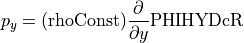
 valid_max: 783.6217041015625
- time: 1
- k: 50
- tile: 13
- j: 90
- i: 90
- dask.array<chunksize=(1, 50, 13, 90, 90), meta=np.ndarray>
Array Chunk Bytes 20.08 MiB 20.08 MiB Shape (1, 50, 13, 90, 90) (1, 50, 13, 90, 90) Count 2 Tasks 1 Chunks Type float32 numpy.ndarray - i(i)int320 1 2 3 4 5 6 ... 84 85 86 87 88 89
- axis :
- X
- long_name :
- grid index in x for variables at tracer and 'v' locations
- swap_dim :
- XC
- comment :
- In the Arakawa C-grid system, tracer (e.g., THETA) and 'v' variables (e.g., VVEL) have the same x coordinate on the model grid.
- coverage_content_type :
- coordinate
array([ 0, 1, 2, 3, 4, 5, 6, 7, 8, 9, 10, 11, 12, 13, 14, 15, 16, 17, 18, 19, 20, 21, 22, 23, 24, 25, 26, 27, 28, 29, 30, 31, 32, 33, 34, 35, 36, 37, 38, 39, 40, 41, 42, 43, 44, 45, 46, 47, 48, 49, 50, 51, 52, 53, 54, 55, 56, 57, 58, 59, 60, 61, 62, 63, 64, 65, 66, 67, 68, 69, 70, 71, 72, 73, 74, 75, 76, 77, 78, 79, 80, 81, 82, 83, 84, 85, 86, 87, 88, 89])
- j(j)int320 1 2 3 4 5 6 ... 84 85 86 87 88 89
- axis :
- Y
- long_name :
- grid index in y for variables at tracer and 'u' locations
- swap_dim :
- YC
- comment :
- In the Arakawa C-grid system, tracer (e.g., THETA) and 'u' variables (e.g., UVEL) have the same y coordinate on the model grid.
- coverage_content_type :
- coordinate
array([ 0, 1, 2, 3, 4, 5, 6, 7, 8, 9, 10, 11, 12, 13, 14, 15, 16, 17, 18, 19, 20, 21, 22, 23, 24, 25, 26, 27, 28, 29, 30, 31, 32, 33, 34, 35, 36, 37, 38, 39, 40, 41, 42, 43, 44, 45, 46, 47, 48, 49, 50, 51, 52, 53, 54, 55, 56, 57, 58, 59, 60, 61, 62, 63, 64, 65, 66, 67, 68, 69, 70, 71, 72, 73, 74, 75, 76, 77, 78, 79, 80, 81, 82, 83, 84, 85, 86, 87, 88, 89])
- k(k)int320 1 2 3 4 5 6 ... 44 45 46 47 48 49
- axis :
- Z
- long_name :
- grid index in z for tracer variables
- swap_dim :
- Z
- coverage_content_type :
- coordinate
array([ 0, 1, 2, 3, 4, 5, 6, 7, 8, 9, 10, 11, 12, 13, 14, 15, 16, 17, 18, 19, 20, 21, 22, 23, 24, 25, 26, 27, 28, 29, 30, 31, 32, 33, 34, 35, 36, 37, 38, 39, 40, 41, 42, 43, 44, 45, 46, 47, 48, 49])
- tile(tile)int320 1 2 3 4 5 6 7 8 9 10 11 12
- long_name :
- lat-lon-cap tile index
- comment :
- The ECCO V4 horizontal model grid is divided into 13 tiles of 90x90 cells for convenience.
- coverage_content_type :
- coordinate
array([ 0, 1, 2, 3, 4, 5, 6, 7, 8, 9, 10, 11, 12])
- time(time)datetime64[ns]2000-01-16T12:00:00
- long_name :
- center time of averaging period
- axis :
- T
- bounds :
- time_bnds
- coverage_content_type :
- coordinate
- standard_name :
- time
array(['2000-01-16T12:00:00.000000000'], dtype='datetime64[ns]')
- XC(tile, j, i)float32dask.array<chunksize=(13, 90, 90), meta=np.ndarray>
- long_name :
- longitude of tracer grid cell center
- units :
- degrees_east
- coordinate :
- YC XC
- bounds :
- XC_bnds
- comment :
- nonuniform grid spacing
- coverage_content_type :
- coordinate
- standard_name :
- longitude
Array Chunk Bytes 411.33 kiB 411.33 kiB Shape (13, 90, 90) (13, 90, 90) Count 2 Tasks 1 Chunks Type float32 numpy.ndarray - YC(tile, j, i)float32dask.array<chunksize=(13, 90, 90), meta=np.ndarray>
- long_name :
- latitude of tracer grid cell center
- units :
- degrees_north
- coordinate :
- YC XC
- bounds :
- YC_bnds
- comment :
- nonuniform grid spacing
- coverage_content_type :
- coordinate
- standard_name :
- latitude
Array Chunk Bytes 411.33 kiB 411.33 kiB Shape (13, 90, 90) (13, 90, 90) Count 2 Tasks 1 Chunks Type float32 numpy.ndarray - Z(k)float32dask.array<chunksize=(50,), meta=np.ndarray>
- long_name :
- depth of tracer grid cell center
- units :
- m
- positive :
- up
- bounds :
- Z_bnds
- comment :
- Non-uniform vertical spacing.
- coverage_content_type :
- coordinate
- standard_name :
- depth
Array Chunk Bytes 200 B 200 B Shape (50,) (50,) Count 2 Tasks 1 Chunks Type float32 numpy.ndarray
- long_name :
- Ocean hydrostatic pressure anomaly at constant depths
- units :
- m2 s-2
- coverage_content_type :
- modelResult
- comment :
- PHIHYD = p(k) / rhoConst - g z(k,t), where p = hydrostatic ocean pressure at depth level k, rhoConst = reference density (1029 kg m-3), g is acceleration due to gravity (9.81 m s-2), and z(k,t) is fixed model depth at level k. Units: p:[kg m-1 s-2], rhoConst:[kg m-3], g:[m s-2], H(t):[m]. Note: includes atmospheric pressure loading. Quantity referred to in some contexts as hydrostatic pressure potential anomaly. PHIHYDcR is calculated with respect to the model's initial, time-invariant grid cell thicknesses. See PHIHYD for hydrostatic pressure anomaly calculated using model's time-variable grid cell thicknesses (z* coordinate system). PHIHYDcR is is NOT corrected for global mean steric sea level changes related to density changes in the Boussinesq volume-conserving model (Greatbatch correction, see sterGloH).
- valid_min :
- 78.17041778564453
- valid_max :
- 783.6217041015625
That’s a long comment! But what we need to know is that PHIHYDcR is related to the actual in-situ ocean pressure by
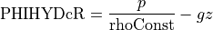
where is a depth coordinate, and rhoConst and are constants. Therefore, the term does not impact the computation of horizontal gradients of pressure, which is what we need for geostrophic balance.
Look at velocity file
Lastly we will need the actual ECCO velocity fields to compute the other side of the geostrophic balance equations. The files in the velocity dataset have 3 data variables (UVEL,VVEL,WVEL) corresponding to the components of three-dimensional velocities. You’ll notice that the velocity fields are each centered in a different location corresponding to an outer face of a grid cell, rather than the center (since the output is from an Arakawa C-grid model).
[14]:
# locate files to load
download_root_dir = join(user_home_dir,'Downloads','ECCO_V4r4_PODAAC')
download_dir = join(download_root_dir,vel_monthly_shortname)
curr_vel_files = list(glob.glob(join(download_dir,'*nc')))
print(f'number of files to load: {len(curr_vel_files)}')
# load file into workspace
# (in this case only 1 file, but this function can load multiple netCDF files with compatible dimensions)
ds_vel_mo = xr.open_mfdataset(curr_vel_files, parallel=True, data_vars='minimal',\
coords='minimal', compat='override')
# check the variables and their associated units
ds_vel_mo
number of files to load: 1
[14]:
<xarray.Dataset> Dimensions: (i: 90, i_g: 90, j: 90, j_g: 90, k: 50, k_u: 50, k_l: 50, k_p1: 51, tile: 13, time: 1, nv: 2, nb: 4) Coordinates: (12/22) * i (i) int32 0 1 2 3 4 5 6 7 8 9 ... 80 81 82 83 84 85 86 87 88 89 * i_g (i_g) int32 0 1 2 3 4 5 6 7 8 9 ... 80 81 82 83 84 85 86 87 88 89 * j (j) int32 0 1 2 3 4 5 6 7 8 9 ... 80 81 82 83 84 85 86 87 88 89 * j_g (j_g) int32 0 1 2 3 4 5 6 7 8 9 ... 80 81 82 83 84 85 86 87 88 89 * k (k) int32 0 1 2 3 4 5 6 7 8 9 ... 40 41 42 43 44 45 46 47 48 49 * k_u (k_u) int32 0 1 2 3 4 5 6 7 8 9 ... 40 41 42 43 44 45 46 47 48 49 ... ... Zu (k_u) float32 dask.array<chunksize=(50,), meta=np.ndarray> Zl (k_l) float32 dask.array<chunksize=(50,), meta=np.ndarray> time_bnds (time, nv) datetime64[ns] dask.array<chunksize=(1, 2), meta=np.ndarray> XC_bnds (tile, j, i, nb) float32 dask.array<chunksize=(13, 90, 90, 4), meta=np.ndarray> YC_bnds (tile, j, i, nb) float32 dask.array<chunksize=(13, 90, 90, 4), meta=np.ndarray> Z_bnds (k, nv) float32 dask.array<chunksize=(50, 2), meta=np.ndarray> Dimensions without coordinates: nv, nb Data variables: UVEL (time, k, tile, j, i_g) float32 dask.array<chunksize=(1, 50, 13, 90, 90), meta=np.ndarray> VVEL (time, k, tile, j_g, i) float32 dask.array<chunksize=(1, 50, 13, 90, 90), meta=np.ndarray> WVEL (time, k_l, tile, j, i) float32 dask.array<chunksize=(1, 50, 13, 90, 90), meta=np.ndarray> Attributes: (12/62) acknowledgement: This research was carried out by the Jet... author: Ian Fenty and Ou Wang cdm_data_type: Grid comment: Fields provided on the curvilinear lat-l... Conventions: CF-1.8, ACDD-1.3 coordinates_comment: Note: the global 'coordinates' attribute... ... ... time_coverage_duration: P1M time_coverage_end: 2000-02-01T00:00:00 time_coverage_resolution: P1M time_coverage_start: 2000-01-01T00:00:00 title: ECCO Ocean Velocity - Monthly Mean llc90... uuid: 32bd652c-4182-11eb-bd5c-0cc47a3f82e7
- i: 90
- i_g: 90
- j: 90
- j_g: 90
- k: 50
- k_u: 50
- k_l: 50
- k_p1: 51
- tile: 13
- time: 1
- nv: 2
- nb: 4
- i(i)int320 1 2 3 4 5 6 ... 84 85 86 87 88 89
- axis :
- X
- long_name :
- grid index in x for variables at tracer and 'v' locations
- swap_dim :
- XC
- comment :
- In the Arakawa C-grid system, tracer (e.g., THETA) and 'v' variables (e.g., VVEL) have the same x coordinate on the model grid.
- coverage_content_type :
- coordinate
array([ 0, 1, 2, 3, 4, 5, 6, 7, 8, 9, 10, 11, 12, 13, 14, 15, 16, 17, 18, 19, 20, 21, 22, 23, 24, 25, 26, 27, 28, 29, 30, 31, 32, 33, 34, 35, 36, 37, 38, 39, 40, 41, 42, 43, 44, 45, 46, 47, 48, 49, 50, 51, 52, 53, 54, 55, 56, 57, 58, 59, 60, 61, 62, 63, 64, 65, 66, 67, 68, 69, 70, 71, 72, 73, 74, 75, 76, 77, 78, 79, 80, 81, 82, 83, 84, 85, 86, 87, 88, 89])
- i_g(i_g)int320 1 2 3 4 5 6 ... 84 85 86 87 88 89
- axis :
- X
- long_name :
- grid index in x for variables at 'u' and 'g' locations
- c_grid_axis_shift :
- -0.5
- swap_dim :
- XG
- comment :
- In the Arakawa C-grid system, 'u' (e.g., UVEL) and 'g' variables (e.g., XG) have the same x coordinate on the model grid.
- coverage_content_type :
- coordinate
array([ 0, 1, 2, 3, 4, 5, 6, 7, 8, 9, 10, 11, 12, 13, 14, 15, 16, 17, 18, 19, 20, 21, 22, 23, 24, 25, 26, 27, 28, 29, 30, 31, 32, 33, 34, 35, 36, 37, 38, 39, 40, 41, 42, 43, 44, 45, 46, 47, 48, 49, 50, 51, 52, 53, 54, 55, 56, 57, 58, 59, 60, 61, 62, 63, 64, 65, 66, 67, 68, 69, 70, 71, 72, 73, 74, 75, 76, 77, 78, 79, 80, 81, 82, 83, 84, 85, 86, 87, 88, 89])
- j(j)int320 1 2 3 4 5 6 ... 84 85 86 87 88 89
- axis :
- Y
- long_name :
- grid index in y for variables at tracer and 'u' locations
- swap_dim :
- YC
- comment :
- In the Arakawa C-grid system, tracer (e.g., THETA) and 'u' variables (e.g., UVEL) have the same y coordinate on the model grid.
- coverage_content_type :
- coordinate
array([ 0, 1, 2, 3, 4, 5, 6, 7, 8, 9, 10, 11, 12, 13, 14, 15, 16, 17, 18, 19, 20, 21, 22, 23, 24, 25, 26, 27, 28, 29, 30, 31, 32, 33, 34, 35, 36, 37, 38, 39, 40, 41, 42, 43, 44, 45, 46, 47, 48, 49, 50, 51, 52, 53, 54, 55, 56, 57, 58, 59, 60, 61, 62, 63, 64, 65, 66, 67, 68, 69, 70, 71, 72, 73, 74, 75, 76, 77, 78, 79, 80, 81, 82, 83, 84, 85, 86, 87, 88, 89])
- j_g(j_g)int320 1 2 3 4 5 6 ... 84 85 86 87 88 89
- axis :
- Y
- long_name :
- grid index in y for variables at 'v' and 'g' locations
- c_grid_axis_shift :
- -0.5
- swap_dim :
- YG
- comment :
- In the Arakawa C-grid system, 'v' (e.g., VVEL) and 'g' variables (e.g., XG) have the same y coordinate.
- coverage_content_type :
- coordinate
array([ 0, 1, 2, 3, 4, 5, 6, 7, 8, 9, 10, 11, 12, 13, 14, 15, 16, 17, 18, 19, 20, 21, 22, 23, 24, 25, 26, 27, 28, 29, 30, 31, 32, 33, 34, 35, 36, 37, 38, 39, 40, 41, 42, 43, 44, 45, 46, 47, 48, 49, 50, 51, 52, 53, 54, 55, 56, 57, 58, 59, 60, 61, 62, 63, 64, 65, 66, 67, 68, 69, 70, 71, 72, 73, 74, 75, 76, 77, 78, 79, 80, 81, 82, 83, 84, 85, 86, 87, 88, 89])
- k(k)int320 1 2 3 4 5 6 ... 44 45 46 47 48 49
- axis :
- Z
- long_name :
- grid index in z for tracer variables
- swap_dim :
- Z
- coverage_content_type :
- coordinate
array([ 0, 1, 2, 3, 4, 5, 6, 7, 8, 9, 10, 11, 12, 13, 14, 15, 16, 17, 18, 19, 20, 21, 22, 23, 24, 25, 26, 27, 28, 29, 30, 31, 32, 33, 34, 35, 36, 37, 38, 39, 40, 41, 42, 43, 44, 45, 46, 47, 48, 49])
- k_u(k_u)int320 1 2 3 4 5 6 ... 44 45 46 47 48 49
- axis :
- Z
- c_grid_axis_shift :
- 0.5
- swap_dim :
- Zu
- coverage_content_type :
- coordinate
- long_name :
- grid index in z corresponding to the bottom face of tracer grid cells ('w' locations)
- comment :
- First index corresponds to the bottom surface of the uppermost tracer grid cell. The use of 'u' in the variable name follows the MITgcm convention for ocean variables in which the upper (u) face of a tracer grid cell on the logical grid corresponds to the bottom face of the grid cell on the physical grid.
array([ 0, 1, 2, 3, 4, 5, 6, 7, 8, 9, 10, 11, 12, 13, 14, 15, 16, 17, 18, 19, 20, 21, 22, 23, 24, 25, 26, 27, 28, 29, 30, 31, 32, 33, 34, 35, 36, 37, 38, 39, 40, 41, 42, 43, 44, 45, 46, 47, 48, 49])
- k_l(k_l)int320 1 2 3 4 5 6 ... 44 45 46 47 48 49
- axis :
- Z
- c_grid_axis_shift :
- -0.5
- swap_dim :
- Zl
- coverage_content_type :
- coordinate
- long_name :
- grid index in z corresponding to the top face of tracer grid cells ('w' locations)
- comment :
- First index corresponds to the top surface of the uppermost tracer grid cell. The use of 'l' in the variable name follows the MITgcm convention for ocean variables in which the lower (l) face of a tracer grid cell on the logical grid corresponds to the top face of the grid cell on the physical grid.
array([ 0, 1, 2, 3, 4, 5, 6, 7, 8, 9, 10, 11, 12, 13, 14, 15, 16, 17, 18, 19, 20, 21, 22, 23, 24, 25, 26, 27, 28, 29, 30, 31, 32, 33, 34, 35, 36, 37, 38, 39, 40, 41, 42, 43, 44, 45, 46, 47, 48, 49])
- k_p1(k_p1)int320 1 2 3 4 5 6 ... 45 46 47 48 49 50
- axis :
- Z
- long_name :
- grid index in z for variables at 'w' locations
- c_grid_axis_shift :
- [-0.5 0.5]
- swap_dim :
- Zp1
- comment :
- Includes top of uppermost model tracer cell (k_p1=0) and bottom of lowermost tracer cell (k_p1=51).
- coverage_content_type :
- coordinate
array([ 0, 1, 2, 3, 4, 5, 6, 7, 8, 9, 10, 11, 12, 13, 14, 15, 16, 17, 18, 19, 20, 21, 22, 23, 24, 25, 26, 27, 28, 29, 30, 31, 32, 33, 34, 35, 36, 37, 38, 39, 40, 41, 42, 43, 44, 45, 46, 47, 48, 49, 50])
- tile(tile)int320 1 2 3 4 5 6 7 8 9 10 11 12
- long_name :
- lat-lon-cap tile index
- comment :
- The ECCO V4 horizontal model grid is divided into 13 tiles of 90x90 cells for convenience.
- coverage_content_type :
- coordinate
array([ 0, 1, 2, 3, 4, 5, 6, 7, 8, 9, 10, 11, 12])
- time(time)datetime64[ns]2000-01-16T12:00:00
- long_name :
- center time of averaging period
- axis :
- T
- bounds :
- time_bnds
- coverage_content_type :
- coordinate
- standard_name :
- time
array(['2000-01-16T12:00:00.000000000'], dtype='datetime64[ns]')
- XC(tile, j, i)float32dask.array<chunksize=(13, 90, 90), meta=np.ndarray>
- long_name :
- longitude of tracer grid cell center
- units :
- degrees_east
- coordinate :
- YC XC
- bounds :
- XC_bnds
- comment :
- nonuniform grid spacing
- coverage_content_type :
- coordinate
- standard_name :
- longitude
Array Chunk Bytes 411.33 kiB 411.33 kiB Shape (13, 90, 90) (13, 90, 90) Count 2 Tasks 1 Chunks Type float32 numpy.ndarray - YC(tile, j, i)float32dask.array<chunksize=(13, 90, 90), meta=np.ndarray>
- long_name :
- latitude of tracer grid cell center
- units :
- degrees_north
- coordinate :
- YC XC
- bounds :
- YC_bnds
- comment :
- nonuniform grid spacing
- coverage_content_type :
- coordinate
- standard_name :
- latitude
Array Chunk Bytes 411.33 kiB 411.33 kiB Shape (13, 90, 90) (13, 90, 90) Count 2 Tasks 1 Chunks Type float32 numpy.ndarray - XG(tile, j_g, i_g)float32dask.array<chunksize=(13, 90, 90), meta=np.ndarray>
- long_name :
- longitude of 'southwest' corner of tracer grid cell
- units :
- degrees_east
- coordinate :
- YG XG
- comment :
- Nonuniform grid spacing. Note: 'southwest' does not correspond to geographic orientation but is used for convenience to describe the computational grid. See MITgcm dcoumentation for details.
- coverage_content_type :
- coordinate
- standard_name :
- longitude
Array Chunk Bytes 411.33 kiB 411.33 kiB Shape (13, 90, 90) (13, 90, 90) Count 2 Tasks 1 Chunks Type float32 numpy.ndarray - YG(tile, j_g, i_g)float32dask.array<chunksize=(13, 90, 90), meta=np.ndarray>
- long_name :
- latitude of 'southwest' corner of tracer grid cell
- units :
- degrees_north
- coordinate :
- YG XG
- comment :
- Nonuniform grid spacing. Note: 'southwest' does not correspond to geographic orientation but is used for convenience to describe the computational grid. See MITgcm dcoumentation for details.
- coverage_content_type :
- coordinate
- standard_name :
- latitude
Array Chunk Bytes 411.33 kiB 411.33 kiB Shape (13, 90, 90) (13, 90, 90) Count 2 Tasks 1 Chunks Type float32 numpy.ndarray - Z(k)float32dask.array<chunksize=(50,), meta=np.ndarray>
- long_name :
- depth of tracer grid cell center
- units :
- m
- positive :
- up
- bounds :
- Z_bnds
- comment :
- Non-uniform vertical spacing.
- coverage_content_type :
- coordinate
- standard_name :
- depth
Array Chunk Bytes 200 B 200 B Shape (50,) (50,) Count 2 Tasks 1 Chunks Type float32 numpy.ndarray - Zp1(k_p1)float32dask.array<chunksize=(51,), meta=np.ndarray>
- long_name :
- depth of tracer grid cell interface
- units :
- m
- positive :
- up
- comment :
- Contains one element more than the number of vertical layers. First element is 0m, the depth of the upper interface of the surface grid cell. Last element is the depth of the lower interface of the deepest grid cell.
- coverage_content_type :
- coordinate
- standard_name :
- depth
Array Chunk Bytes 204 B 204 B Shape (51,) (51,) Count 2 Tasks 1 Chunks Type float32 numpy.ndarray - Zu(k_u)float32dask.array<chunksize=(50,), meta=np.ndarray>
- units :
- m
- positive :
- up
- coverage_content_type :
- coordinate
- standard_name :
- depth
- long_name :
- depth of the bottom face of tracer grid cells
- comment :
- First element is -10m, the depth of the bottom face of the first tracer grid cell. Last element is the depth of the bottom face of the deepest grid cell. The use of 'u' in the variable name follows the MITgcm convention for ocean variables in which the upper (u) face of a tracer grid cell on the logical grid corresponds to the bottom face of the grid cell on the physical grid. In other words, the logical vertical grid of MITgcm ocean variables is inverted relative to the physical vertical grid.
Array Chunk Bytes 200 B 200 B Shape (50,) (50,) Count 2 Tasks 1 Chunks Type float32 numpy.ndarray - Zl(k_l)float32dask.array<chunksize=(50,), meta=np.ndarray>
- units :
- m
- positive :
- up
- coverage_content_type :
- coordinate
- standard_name :
- depth
- long_name :
- depth of the top face of tracer grid cells
- comment :
- First element is 0m, the depth of the top face of the first tracer grid cell (ocean surface). Last element is the depth of the top face of the deepest grid cell. The use of 'l' in the variable name follows the MITgcm convention for ocean variables in which the lower (l) face of a tracer grid cell on the logical grid corresponds to the top face of the grid cell on the physical grid. In other words, the logical vertical grid of MITgcm ocean variables is inverted relative to the physical vertical grid.
Array Chunk Bytes 200 B 200 B Shape (50,) (50,) Count 2 Tasks 1 Chunks Type float32 numpy.ndarray - time_bnds(time, nv)datetime64[ns]dask.array<chunksize=(1, 2), meta=np.ndarray>
- comment :
- Start and end times of averaging period.
- coverage_content_type :
- coordinate
- long_name :
- time bounds of averaging period
Array Chunk Bytes 16 B 16 B Shape (1, 2) (1, 2) Count 2 Tasks 1 Chunks Type datetime64[ns] numpy.ndarray - XC_bnds(tile, j, i, nb)float32dask.array<chunksize=(13, 90, 90, 4), meta=np.ndarray>
- comment :
- Bounds array follows CF conventions. XC_bnds[i,j,0] = 'southwest' corner (j-1, i-1), XC_bnds[i,j,1] = 'southeast' corner (j-1, i+1), XC_bnds[i,j,2] = 'northeast' corner (j+1, i+1), XC_bnds[i,j,3] = 'northwest' corner (j+1, i-1). Note: 'southwest', 'southeast', northwest', and 'northeast' do not correspond to geographic orientation but are used for convenience to describe the computational grid. See MITgcm dcoumentation for details.
- coverage_content_type :
- coordinate
- long_name :
- longitudes of tracer grid cell corners
Array Chunk Bytes 1.61 MiB 1.61 MiB Shape (13, 90, 90, 4) (13, 90, 90, 4) Count 2 Tasks 1 Chunks Type float32 numpy.ndarray - YC_bnds(tile, j, i, nb)float32dask.array<chunksize=(13, 90, 90, 4), meta=np.ndarray>
- comment :
- Bounds array follows CF conventions. YC_bnds[i,j,0] = 'southwest' corner (j-1, i-1), YC_bnds[i,j,1] = 'southeast' corner (j-1, i+1), YC_bnds[i,j,2] = 'northeast' corner (j+1, i+1), YC_bnds[i,j,3] = 'northwest' corner (j+1, i-1). Note: 'southwest', 'southeast', northwest', and 'northeast' do not correspond to geographic orientation but are used for convenience to describe the computational grid. See MITgcm dcoumentation for details.
- coverage_content_type :
- coordinate
- long_name :
- latitudes of tracer grid cell corners
Array Chunk Bytes 1.61 MiB 1.61 MiB Shape (13, 90, 90, 4) (13, 90, 90, 4) Count 2 Tasks 1 Chunks Type float32 numpy.ndarray - Z_bnds(k, nv)float32dask.array<chunksize=(50, 2), meta=np.ndarray>
- comment :
- One pair of depths for each vertical level.
- coverage_content_type :
- coordinate
- long_name :
- depths of tracer grid cell upper and lower interfaces
Array Chunk Bytes 400 B 400 B Shape (50, 2) (50, 2) Count 2 Tasks 1 Chunks Type float32 numpy.ndarray
- UVEL(time, k, tile, j, i_g)float32dask.array<chunksize=(1, 50, 13, 90, 90), meta=np.ndarray>
- long_name :
- Horizontal velocity in the model +x direction
- units :
- m s-1
- mate :
- VVEL
- coverage_content_type :
- modelResult
- direction :
- >0 increases volume
- standard_name :
- sea_water_x_velocity
- comment :
- Horizontal velocity in the +x direction at the 'u' face of the tracer cell on the native model grid. Note: in the Arakawa-C grid, horizontal velocities are staggered relative to the tracer cells with indexing such that +UVEL(i_g,j,k) corresponds to +x fluxes through the 'u' face of the tracer cell at (i,j,k). Do NOT use UVEL for volume flux calculations because the model's grid cell thicknesses vary with time (z* coordinates); use UVELMASS instead. Also, the model +x direction does not necessarily correspond to the geographical east-west direction because the x and y axes of the model's curvilinear lat-lon-cap (llc) grid have arbitrary orientations which vary within and across tiles. See EVEL and NVEL for zonal and meridional velocity.
- valid_min :
- -1.2937312126159668
- valid_max :
- 1.776294231414795
Array Chunk Bytes 20.08 MiB 20.08 MiB Shape (1, 50, 13, 90, 90) (1, 50, 13, 90, 90) Count 2 Tasks 1 Chunks Type float32 numpy.ndarray - VVEL(time, k, tile, j_g, i)float32dask.array<chunksize=(1, 50, 13, 90, 90), meta=np.ndarray>
- long_name :
- Horizontal velocity in the model +y direction
- units :
- m s-1
- mate :
- UVEL
- coverage_content_type :
- modelResult
- direction :
- >0 increases volume
- standard_name :
- sea_water_y_velocity
- comment :
- Horizontal velocity in the +y direction at the 'v' face of the tracer cell on the native model grid. Note: in the Arakawa-C grid, horizontal velocities are staggered relative to the tracer cells with indexing such that +VVEL(i,j_g,k) corresponds to +y fluxes through the 'v' face of the tracer cell at (i,j,k). Do NOT use VVEL for volume flux calculations because the model's grid cell thicknesses vary with time (z* coordinates); use VVELMASS instead. Also, the model +y direction does not necessarily correspond to the geographical north-south direction because the x and y axes of the model's curvilinear lat-lon-cap (llc) grid have arbitrary orientations which vary within and across tiles. See EVEL and NVEL for zonal and meridional velocity.
- valid_min :
- -1.2608345746994019
- valid_max :
- 1.4756959676742554
Array Chunk Bytes 20.08 MiB 20.08 MiB Shape (1, 50, 13, 90, 90) (1, 50, 13, 90, 90) Count 2 Tasks 1 Chunks Type float32 numpy.ndarray - WVEL(time, k_l, tile, j, i)float32dask.array<chunksize=(1, 50, 13, 90, 90), meta=np.ndarray>
- long_name :
- Vertical velocity
- units :
- m s-1
- coverage_content_type :
- modelResult
- direction :
- >0 decreases volume
- standard_name :
- upward_sea_water_velocity
- comment :
- Vertical velocity in the +z direction at the top 'w' face of the tracer cell on the native model grid. Note: in the Arakawa-C grid, vertical velocities are staggered relative to the tracer cells with indexing such that +WVEL(i,j,k_l) corresponds to upward +z motion through the top 'w' face of the tracer cell at (i,j,k). WVEL is identical to WVELMASS.
- valid_min :
- -0.0012012795777991414
- valid_max :
- 0.0005706523661501706
Array Chunk Bytes 20.08 MiB 20.08 MiB Shape (1, 50, 13, 90, 90) (1, 50, 13, 90, 90) Count 2 Tasks 1 Chunks Type float32 numpy.ndarray
- acknowledgement :
- This research was carried out by the Jet Propulsion Laboratory, managed by the California Institute of Technology under a contract with the National Aeronautics and Space Administration.
- author :
- Ian Fenty and Ou Wang
- cdm_data_type :
- Grid
- comment :
- Fields provided on the curvilinear lat-lon-cap 90 (llc90) native grid used in the ECCO model.
- Conventions :
- CF-1.8, ACDD-1.3
- coordinates_comment :
- Note: the global 'coordinates' attribute describes auxillary coordinates.
- creator_email :
- ecco-group@mit.edu
- creator_institution :
- NASA Jet Propulsion Laboratory (JPL)
- creator_name :
- ECCO Consortium
- creator_type :
- group
- creator_url :
- https://ecco-group.org
- date_created :
- 2020-12-18T14:41:41
- date_issued :
- 2020-12-18T14:41:41
- date_metadata_modified :
- 2021-03-15T21:55:00
- date_modified :
- 2021-03-15T21:55:00
- geospatial_bounds_crs :
- EPSG:4326
- geospatial_lat_max :
- 90.0
- geospatial_lat_min :
- -90.0
- geospatial_lat_resolution :
- variable
- geospatial_lat_units :
- degrees_north
- geospatial_lon_max :
- 180.0
- geospatial_lon_min :
- -180.0
- geospatial_lon_resolution :
- variable
- geospatial_lon_units :
- degrees_east
- geospatial_vertical_max :
- 0.0
- geospatial_vertical_min :
- -6134.5
- geospatial_vertical_positive :
- up
- geospatial_vertical_resolution :
- variable
- geospatial_vertical_units :
- meter
- history :
- Inaugural release of an ECCO Central Estimate solution to PO.DAAC
- id :
- 10.5067/ECL5M-OVE44
- institution :
- NASA Jet Propulsion Laboratory (JPL)
- instrument_vocabulary :
- GCMD instrument keywords
- keywords :
- EARTH SCIENCE > OCEANS > OCEAN CIRCULATION, EARTH SCIENCE SERVICES > MODELS > EARTH SCIENCE REANALYSES/ASSIMILATION MODELS, EARTH SCIENCE > OCEANS > OCEAN CIRCULATION > OCEAN CURRENTS
- keywords_vocabulary :
- NASA Global Change Master Directory (GCMD) Science Keywords
- license :
- Public Domain
- metadata_link :
- https://cmr.earthdata.nasa.gov/search/collections.umm_json?ShortName=ECCO_L4_OCEAN_VEL_LLC0090GRID_MONTHLY_V4R4
- naming_authority :
- gov.nasa.jpl
- platform :
- ERS-1/2, TOPEX/Poseidon, Geosat Follow-On (GFO), ENVISAT, Jason-1, Jason-2, CryoSat-2, SARAL/AltiKa, Jason-3, AVHRR, Aquarius, SSM/I, SSMIS, GRACE, DTU17MDT, Argo, WOCE, GO-SHIP, MEOP, Ice Tethered Profilers (ITP)
- platform_vocabulary :
- GCMD platform keywords
- processing_level :
- L4
- product_name :
- OCEAN_VELOCITY_mon_mean_2000-01_ECCO_V4r4_native_llc0090.nc
- product_time_coverage_end :
- 2018-01-01T00:00:00
- product_time_coverage_start :
- 1992-01-01T12:00:00
- product_version :
- Version 4, Release 4
- program :
- NASA Physical Oceanography, Cryosphere, Modeling, Analysis, and Prediction (MAP)
- project :
- Estimating the Circulation and Climate of the Ocean (ECCO)
- publisher_email :
- podaac@podaac.jpl.nasa.gov
- publisher_institution :
- PO.DAAC
- publisher_name :
- Physical Oceanography Distributed Active Archive Center (PO.DAAC)
- publisher_type :
- institution
- publisher_url :
- https://podaac.jpl.nasa.gov
- references :
- ECCO Consortium, Fukumori, I., Wang, O., Fenty, I., Forget, G., Heimbach, P., & Ponte, R. M. 2020. Synopsis of the ECCO Central Production Global Ocean and Sea-Ice State Estimate (Version 4 Release 4). doi:10.5281/zenodo.3765928
- source :
- The ECCO V4r4 state estimate was produced by fitting a free-running solution of the MITgcm (checkpoint 66g) to satellite and in situ observational data in a least squares sense using the adjoint method
- standard_name_vocabulary :
- NetCDF Climate and Forecast (CF) Metadata Convention
- summary :
- This dataset provides monthly-averaged ocean velocity on the lat-lon-cap 90 (llc90) native model grid from the ECCO Version 4 Release 4 (V4r4) ocean and sea-ice state estimate. Estimating the Circulation and Climate of the Ocean (ECCO) state estimates are dynamically and kinematically-consistent reconstructions of the three-dimensional, time-evolving ocean, sea-ice, and surface atmospheric states. ECCO V4r4 is a free-running solution of a global, nominally 1-degree configuration of the MIT general circulation model (MITgcm) that has been fit to observations in a least-squares sense. Observational data constraints used in V4r4 include sea surface height (SSH) from satellite altimeters [ERS-1/2, TOPEX/Poseidon, GFO, ENVISAT, Jason-1,2,3, CryoSat-2, and SARAL/AltiKa]; sea surface temperature (SST) from satellite radiometers [AVHRR], sea surface salinity (SSS) from the Aquarius satellite radiometer/scatterometer, ocean bottom pressure (OBP) from the GRACE satellite gravimeter; sea-ice concentration from satellite radiometers [SSM/I and SSMIS], and in-situ ocean temperature and salinity measured with conductivity-temperature-depth (CTD) sensors and expendable bathythermographs (XBTs) from several programs [e.g., WOCE, GO-SHIP, Argo, and others] and platforms [e.g., research vessels, gliders, moorings, ice-tethered profilers, and instrumented pinnipeds]. V4r4 covers the period 1992-01-01T12:00:00 to 2018-01-01T00:00:00.
- time_coverage_duration :
- P1M
- time_coverage_end :
- 2000-02-01T00:00:00
- time_coverage_resolution :
- P1M
- time_coverage_start :
- 2000-01-01T00:00:00
- title :
- ECCO Ocean Velocity - Monthly Mean llc90 Grid (Version 4 Release 4)
- uuid :
- 32bd652c-4182-11eb-bd5c-0cc47a3f82e7
Compute and map geostrophic balance
Now that we are aware of the corrections needed to get actual in-situ density and pressure (gradients) from ECCO, we are ready to assess geostrophic balance. Let’s consider the k=20
depth level again; we are deliberately avoiding plotting at the surface for reasons that will be apparent later!
The right-hand side of the geostrophic balance equations are and , and and can be computed as
with .
Now we load the grid parameters to help us compute derivatives:
[15]:
grid_params_shortname = "ECCO_L4_GEOMETRY_LLC0090GRID_V4R4"
grid_params_file = "GRID_GEOMETRY_ECCO_V4r4_native_llc0090.nc"
grid_params_file_path = join(download_root_dir,grid_params_shortname,grid_params_file)
# load grid parameters file
ds_grid = xr.open_dataset(grid_params_file_path)
ds_grid
[15]:
<xarray.Dataset> Dimensions: (i: 90, i_g: 90, j: 90, j_g: 90, k: 50, k_u: 50, k_l: 50, k_p1: 51, tile: 13, nb: 4, nv: 2) Coordinates: (12/20) * i (i) int32 0 1 2 3 4 5 6 7 8 9 10 ... 80 81 82 83 84 85 86 87 88 89 * i_g (i_g) int32 0 1 2 3 4 5 6 7 8 9 ... 80 81 82 83 84 85 86 87 88 89 * j (j) int32 0 1 2 3 4 5 6 7 8 9 10 ... 80 81 82 83 84 85 86 87 88 89 * j_g (j_g) int32 0 1 2 3 4 5 6 7 8 9 ... 80 81 82 83 84 85 86 87 88 89 * k (k) int32 0 1 2 3 4 5 6 7 8 9 10 ... 40 41 42 43 44 45 46 47 48 49 * k_u (k_u) int32 0 1 2 3 4 5 6 7 8 9 ... 40 41 42 43 44 45 46 47 48 49 ... ... Zp1 (k_p1) float32 0.0 -10.0 -20.0 ... -5.244e+03 -5.678e+03 -6.134e+03 Zu (k_u) float32 -10.0 -20.0 -30.0 ... -5.678e+03 -6.134e+03 Zl (k_l) float32 0.0 -10.0 -20.0 ... -4.834e+03 -5.244e+03 -5.678e+03 XC_bnds (tile, j, i, nb) float32 ... YC_bnds (tile, j, i, nb) float32 ... Z_bnds (k, nv) float32 0.0 -10.0 -10.0 ... -5.678e+03 -6.134e+03 Dimensions without coordinates: nb, nv Data variables: (12/21) CS (tile, j, i) float32 ... SN (tile, j, i) float32 ... rA (tile, j, i) float32 ... dxG (tile, j_g, i) float32 ... dyG (tile, j, i_g) float32 ... Depth (tile, j, i) float32 ... ... ... hFacC (k, tile, j, i) float32 ... hFacW (k, tile, j, i_g) float32 ... hFacS (k, tile, j_g, i) float32 ... maskC (k, tile, j, i) bool ... maskW (k, tile, j, i_g) bool ... maskS (k, tile, j_g, i) bool ... Attributes: (12/58) acknowledgement: This research was carried out by the Jet... author: Ian Fenty and Ou Wang cdm_data_type: Grid comment: Fields provided on the curvilinear lat-l... Conventions: CF-1.8, ACDD-1.3 coordinates_comment: Note: the global 'coordinates' attribute... ... ... references: ECCO Consortium, Fukumori, I., Wang, O.,... source: The ECCO V4r4 state estimate was produce... standard_name_vocabulary: NetCDF Climate and Forecast (CF) Metadat... summary: This dataset provides geometric paramete... title: ECCO Geometry Parameters for the Lat-Lon... uuid: 87ff7d24-86e5-11eb-9c5f-f8f21e2ee3e0
- i: 90
- i_g: 90
- j: 90
- j_g: 90
- k: 50
- k_u: 50
- k_l: 50
- k_p1: 51
- tile: 13
- nb: 4
- nv: 2
- i(i)int320 1 2 3 4 5 6 ... 84 85 86 87 88 89
- axis :
- X
- long_name :
- grid index in x for variables at tracer and 'v' locations
- swap_dim :
- XC
- comment :
- In the Arakawa C-grid system, tracer (e.g., THETA) and 'v' variables (e.g., VVEL) have the same x coordinate on the model grid.
- coverage_content_type :
- coordinate
array([ 0, 1, 2, 3, 4, 5, 6, 7, 8, 9, 10, 11, 12, 13, 14, 15, 16, 17, 18, 19, 20, 21, 22, 23, 24, 25, 26, 27, 28, 29, 30, 31, 32, 33, 34, 35, 36, 37, 38, 39, 40, 41, 42, 43, 44, 45, 46, 47, 48, 49, 50, 51, 52, 53, 54, 55, 56, 57, 58, 59, 60, 61, 62, 63, 64, 65, 66, 67, 68, 69, 70, 71, 72, 73, 74, 75, 76, 77, 78, 79, 80, 81, 82, 83, 84, 85, 86, 87, 88, 89])
- i_g(i_g)int320 1 2 3 4 5 6 ... 84 85 86 87 88 89
- axis :
- X
- long_name :
- grid index in x for variables at 'u' and 'g' locations
- c_grid_axis_shift :
- -0.5
- swap_dim :
- XG
- comment :
- In the Arakawa C-grid system, 'u' (e.g., UVEL) and 'g' variables (e.g., XG) have the same x coordinate on the model grid.
- coverage_content_type :
- coordinate
array([ 0, 1, 2, 3, 4, 5, 6, 7, 8, 9, 10, 11, 12, 13, 14, 15, 16, 17, 18, 19, 20, 21, 22, 23, 24, 25, 26, 27, 28, 29, 30, 31, 32, 33, 34, 35, 36, 37, 38, 39, 40, 41, 42, 43, 44, 45, 46, 47, 48, 49, 50, 51, 52, 53, 54, 55, 56, 57, 58, 59, 60, 61, 62, 63, 64, 65, 66, 67, 68, 69, 70, 71, 72, 73, 74, 75, 76, 77, 78, 79, 80, 81, 82, 83, 84, 85, 86, 87, 88, 89])
- j(j)int320 1 2 3 4 5 6 ... 84 85 86 87 88 89
- axis :
- Y
- long_name :
- grid index in y for variables at tracer and 'u' locations
- swap_dim :
- YC
- comment :
- In the Arakawa C-grid system, tracer (e.g., THETA) and 'u' variables (e.g., UVEL) have the same y coordinate on the model grid.
- coverage_content_type :
- coordinate
array([ 0, 1, 2, 3, 4, 5, 6, 7, 8, 9, 10, 11, 12, 13, 14, 15, 16, 17, 18, 19, 20, 21, 22, 23, 24, 25, 26, 27, 28, 29, 30, 31, 32, 33, 34, 35, 36, 37, 38, 39, 40, 41, 42, 43, 44, 45, 46, 47, 48, 49, 50, 51, 52, 53, 54, 55, 56, 57, 58, 59, 60, 61, 62, 63, 64, 65, 66, 67, 68, 69, 70, 71, 72, 73, 74, 75, 76, 77, 78, 79, 80, 81, 82, 83, 84, 85, 86, 87, 88, 89])
- j_g(j_g)int320 1 2 3 4 5 6 ... 84 85 86 87 88 89
- axis :
- Y
- long_name :
- grid index in y for variables at 'v' and 'g' locations
- c_grid_axis_shift :
- -0.5
- swap_dim :
- YG
- comment :
- In the Arakawa C-grid system, 'v' (e.g., VVEL) and 'g' variables (e.g., XG) have the same y coordinate.
- coverage_content_type :
- coordinate
array([ 0, 1, 2, 3, 4, 5, 6, 7, 8, 9, 10, 11, 12, 13, 14, 15, 16, 17, 18, 19, 20, 21, 22, 23, 24, 25, 26, 27, 28, 29, 30, 31, 32, 33, 34, 35, 36, 37, 38, 39, 40, 41, 42, 43, 44, 45, 46, 47, 48, 49, 50, 51, 52, 53, 54, 55, 56, 57, 58, 59, 60, 61, 62, 63, 64, 65, 66, 67, 68, 69, 70, 71, 72, 73, 74, 75, 76, 77, 78, 79, 80, 81, 82, 83, 84, 85, 86, 87, 88, 89])
- k(k)int320 1 2 3 4 5 6 ... 44 45 46 47 48 49
- axis :
- Z
- long_name :
- grid index in z for tracer variables
- swap_dim :
- Z
- coverage_content_type :
- coordinate
array([ 0, 1, 2, 3, 4, 5, 6, 7, 8, 9, 10, 11, 12, 13, 14, 15, 16, 17, 18, 19, 20, 21, 22, 23, 24, 25, 26, 27, 28, 29, 30, 31, 32, 33, 34, 35, 36, 37, 38, 39, 40, 41, 42, 43, 44, 45, 46, 47, 48, 49])
- k_u(k_u)int320 1 2 3 4 5 6 ... 44 45 46 47 48 49
- axis :
- Z
- long_name :
- grid index in z corresponding to the bottom face of tracer grid cells ('w' locations)
- c_grid_axis_shift :
- 0.5
- swap_dim :
- Zu
- comment :
- First index corresponds to the bottom face of the uppermost tracer grid cell. The use of 'u' in the variable name follows the MITgcm convention for naming the bottom face of ocean tracer grid cells.
- coverage_content_type :
- coordinate
array([ 0, 1, 2, 3, 4, 5, 6, 7, 8, 9, 10, 11, 12, 13, 14, 15, 16, 17, 18, 19, 20, 21, 22, 23, 24, 25, 26, 27, 28, 29, 30, 31, 32, 33, 34, 35, 36, 37, 38, 39, 40, 41, 42, 43, 44, 45, 46, 47, 48, 49])
- k_l(k_l)int320 1 2 3 4 5 6 ... 44 45 46 47 48 49
- axis :
- Z
- long_name :
- grid index in z corresponding to the top face of tracer grid cells ('w' locations)
- c_grid_axis_shift :
- -0.5
- swap_dim :
- Zl
- comment :
- First index corresponds to the top face of the uppermost tracer grid cell. The use of 'l' in the variable name follows the MITgcm convention for naming the top face of ocean tracer grid cells.
- coverage_content_type :
- coordinate
array([ 0, 1, 2, 3, 4, 5, 6, 7, 8, 9, 10, 11, 12, 13, 14, 15, 16, 17, 18, 19, 20, 21, 22, 23, 24, 25, 26, 27, 28, 29, 30, 31, 32, 33, 34, 35, 36, 37, 38, 39, 40, 41, 42, 43, 44, 45, 46, 47, 48, 49])
- k_p1(k_p1)int320 1 2 3 4 5 6 ... 45 46 47 48 49 50
- axis :
- Z
- long_name :
- grid index in z for variables at 'w' locations
- c_grid_axis_shift :
- [-0.5 0.5]
- swap_dim :
- Zp1
- comment :
- Includes top of uppermost model tracer cell (k_p1=0) and bottom of lowermost tracer cell (k_p1=51).
- coverage_content_type :
- coordinate
array([ 0, 1, 2, 3, 4, 5, 6, 7, 8, 9, 10, 11, 12, 13, 14, 15, 16, 17, 18, 19, 20, 21, 22, 23, 24, 25, 26, 27, 28, 29, 30, 31, 32, 33, 34, 35, 36, 37, 38, 39, 40, 41, 42, 43, 44, 45, 46, 47, 48, 49, 50])
- tile(tile)int320 1 2 3 4 5 6 7 8 9 10 11 12
- long_name :
- lat-lon-cap tile index
- comment :
- The ECCO V4 horizontal model grid is divided into 13 tiles of 90x90 cells for convenience.
- coverage_content_type :
- coordinate
array([ 0, 1, 2, 3, 4, 5, 6, 7, 8, 9, 10, 11, 12])
- XC(tile, j, i)float32...
- long_name :
- longitude of tracer grid cell center
- units :
- degrees_east
- coordinate :
- YC XC
- bounds :
- XC_bnds
- comment :
- nonuniform grid spacing
- coverage_content_type :
- coordinate
- standard_name :
- longitude
[105300 values with dtype=float32]
- YC(tile, j, i)float32...
- long_name :
- latitude of tracer grid cell center
- units :
- degrees_north
- coordinate :
- YC XC
- bounds :
- YC_bnds
- comment :
- nonuniform grid spacing
- coverage_content_type :
- coordinate
- standard_name :
- latitude
[105300 values with dtype=float32]
- XG(tile, j_g, i_g)float32...
- long_name :
- longitude of 'southwest' corner of tracer grid cell
- units :
- degrees_east
- coordinate :
- YG XG
- comment :
- Nonuniform grid spacing. Note: 'southwest' does not correspond to geographic orientation but is used for convenience to describe the computational grid. See MITgcm dcoumentation for details.
- coverage_content_type :
- coordinate
- standard_name :
- longitude
[105300 values with dtype=float32]
- YG(tile, j_g, i_g)float32...
- long_name :
- latitude of 'southwest' corner of tracer grid cell
- units :
- degrees_north
- comment :
- Nonuniform grid spacing. Note: 'southwest' does not correspond to geographic orientation but is used for convenience to describe the computational grid. See MITgcm dcoumentation for details.
- coverage_content_type :
- coordinate
- standard_name :
- latitude
[105300 values with dtype=float32]
- Z(k)float32...
- long_name :
- depth of tracer grid cell center
- units :
- m
- positive :
- up
- bounds :
- Z_bnds
- comment :
- Non-uniform vertical spacing.
- coverage_content_type :
- coordinate
- standard_name :
- depth
array([-5.000000e+00, -1.500000e+01, -2.500000e+01, -3.500000e+01, -4.500000e+01, -5.500000e+01, -6.500000e+01, -7.500500e+01, -8.502500e+01, -9.509500e+01, -1.053100e+02, -1.158700e+02, -1.271500e+02, -1.397400e+02, -1.544700e+02, -1.724000e+02, -1.947350e+02, -2.227100e+02, -2.574700e+02, -2.999300e+02, -3.506800e+02, -4.099300e+02, -4.774700e+02, -5.527100e+02, -6.347350e+02, -7.224000e+02, -8.144700e+02, -9.097400e+02, -1.007155e+03, -1.105905e+03, -1.205535e+03, -1.306205e+03, -1.409150e+03, -1.517095e+03, -1.634175e+03, -1.765135e+03, -1.914150e+03, -2.084035e+03, -2.276225e+03, -2.491250e+03, -2.729250e+03, -2.990250e+03, -3.274250e+03, -3.581250e+03, -3.911250e+03, -4.264250e+03, -4.640250e+03, -5.039250e+03, -5.461250e+03, -5.906250e+03], dtype=float32)
- Zp1(k_p1)float32...
- long_name :
- depth of top/bottom face of tracer grid cell
- units :
- m
- positive :
- up
- comment :
- Contains one element more than the number of vertical layers. First element is 0m, the depth of the top face of the uppermost grid cell. Last element is the depth of the bottom face of the deepest grid cell.
- coverage_content_type :
- coordinate
- standard_name :
- depth
array([ 0. , -10. , -20. , -30. , -40. , -50. , -60. , -70. , -80.01, -90.04, -100.15, -110.47, -121.27, -133.03, -146.45, -162.49, -182.31, -207.16, -238.26, -276.68, -323.18, -378.18, -441.68, -513.26, -592.16, -677.31, -767.49, -861.45, -958.03, -1056.28, -1155.53, -1255.54, -1356.87, -1461.43, -1572.76, -1695.59, -1834.68, -1993.62, -2174.45, -2378. , -2604.5 , -2854. , -3126.5 , -3422. , -3740.5 , -4082. , -4446.5 , -4834. , -5244.5 , -5678. , -6134.5 ], dtype=float32)
- Zu(k_u)float32...
- long_name :
- depth of bottom face of tracer grid cell
- units :
- m
- positive :
- up
- comment :
- First element is -10m, the depth of the bottom face of the uppermost tracer grid cell. Last element is the depth of the bottom face of the deepest grid cell. The use of 'u' in the variable name follows the MITgcm convention for naming the bottom face of ocean tracer grid cells.
- coverage_content_type :
- coordinate
- standard_name :
- depth
array([ -10. , -20. , -30. , -40. , -50. , -60. , -70. , -80.01, -90.04, -100.15, -110.47, -121.27, -133.03, -146.45, -162.49, -182.31, -207.16, -238.26, -276.68, -323.18, -378.18, -441.68, -513.26, -592.16, -677.31, -767.49, -861.45, -958.03, -1056.28, -1155.53, -1255.54, -1356.87, -1461.43, -1572.76, -1695.59, -1834.68, -1993.62, -2174.45, -2378. , -2604.5 , -2854. , -3126.5 , -3422. , -3740.5 , -4082. , -4446.5 , -4834. , -5244.5 , -5678. , -6134.5 ], dtype=float32)
- Zl(k_l)float32...
- long_name :
- depth of top face of tracer grid cell
- units :
- m
- positive :
- up
- comment :
- First element is 0m, the depth of the top face of the uppermost tracer grid cell (i.e., the ocean surface). Last element is the depth of the top face of the deepest grid cell. The use of 'l' in the variable name follows the MITgcm convention for naming the top face of ocean tracer grid cells.
- coverage_content_type :
- coordinate
- standard_name :
- depth
array([ 0. , -10. , -20. , -30. , -40. , -50. , -60. , -70. , -80.01, -90.04, -100.15, -110.47, -121.27, -133.03, -146.45, -162.49, -182.31, -207.16, -238.26, -276.68, -323.18, -378.18, -441.68, -513.26, -592.16, -677.31, -767.49, -861.45, -958.03, -1056.28, -1155.53, -1255.54, -1356.87, -1461.43, -1572.76, -1695.59, -1834.68, -1993.62, -2174.45, -2378. , -2604.5 , -2854. , -3126.5 , -3422. , -3740.5 , -4082. , -4446.5 , -4834. , -5244.5 , -5678. ], dtype=float32)
- XC_bnds(tile, j, i, nb)float32...
- comment :
- Bounds array follows CF conventions. XC_bnds[i,j,0] = 'southwest' corner (j-1, i-1), XC_bnds[i,j,1] = 'southeast' corner (j-1, i+1), XC_bnds[i,j,2] = 'northeast' corner (j+1, i+1), XC_bnds[i,j,3] = 'northwest' corner (j+1, i-1). Note: 'southwest', 'southeast', northwest', and 'northeast' do not correspond to geographic orientation but are used for convenience to describe the computational grid. See MITgcm dcoumentation for details.
- coverage_content_type :
- coordinate
- long_name :
- longitudes of tracer grid cell corners
[421200 values with dtype=float32]
- YC_bnds(tile, j, i, nb)float32...
- comment :
- Bounds array follows CF conventions. YC_bnds[i,j,0] = 'southwest' corner (j-1, i-1), YC_bnds[i,j,1] = 'southeast' corner (j-1, i+1), YC_bnds[i,j,2] = 'northeast' corner (j+1, i+1), YC_bnds[i,j,3] = 'northwest' corner (j+1, i-1). Note: 'southwest', 'southeast', northwest', and 'northeast' do not correspond to geographic orientation but are used for convenience to describe the computational grid. See MITgcm dcoumentation for details.
- coverage_content_type :
- coordinate
- long_name :
- latitudes of tracer grid cell corners
[421200 values with dtype=float32]
- Z_bnds(k, nv)float32...
- comment :
- One pair of depths for each vertical level.
- coverage_content_type :
- coordinate
- long_name :
- depths of top and bottom faces of tracer grid cell
array([[ 0. , -10. ], [ -10. , -20. ], [ -20. , -30. ], [ -30. , -40. ], [ -40. , -50. ], [ -50. , -60. ], [ -60. , -70. ], [ -70. , -80.01 ], [ -80.01 , -90.04 ], [ -90.04 , -100.15 ], [ -100.15 , -110.47 ], [ -110.47 , -121.270004], [ -121.270004, -133.03 ], [ -133.03 , -146.45 ], [ -146.45 , -162.48999 ], [ -162.48999 , -182.31 ], [ -182.31 , -207.16 ], [ -207.16 , -238.26001 ], [ -238.26001 , -276.68 ], [ -276.68 , -323.18 ], [ -323.18 , -378.18 ], [ -378.18 , -441.68 ], [ -441.68 , -513.26 ], [ -513.26 , -592.16003 ], [ -592.16003 , -677.31006 ], [ -677.31006 , -767.49005 ], [ -767.49005 , -861.4501 ], [ -861.4501 , -958.0301 ], [ -958.0301 , -1056.28 ], [-1056.28 , -1155.53 ], [-1155.53 , -1255.54 ], [-1255.54 , -1356.87 ], [-1356.87 , -1461.4299 ], [-1461.4299 , -1572.7599 ], [-1572.7599 , -1695.5898 ], [-1695.5898 , -1834.6798 ], [-1834.6798 , -1993.6199 ], [-1993.6199 , -2174.45 ], [-2174.45 , -2378. ], [-2378. , -2604.5 ], [-2604.5 , -2854. ], [-2854. , -3126.5 ], [-3126.5 , -3422. ], [-3422. , -3740.5 ], [-3740.5 , -4082. ], [-4082. , -4446.5 ], [-4446.5 , -4834. ], [-4834. , -5244.5 ], [-5244.5 , -5678. ], [-5678. , -6134.5 ]], dtype=float32)
- CS(tile, j, i)float32...
- long_name :
- cosine of tracer grid cell orientation vs geographical north
- units :
- 1
- coordinate :
- YC XC
- coverage_content_type :
- modelResult
- comment :
- CS and SN are required to calculate the geographic (meridional, zonal) components of vectors on the curvilinear model grid. Note: for vector R with components R_x and R_y: R_{east} = CS R_x - SN R_y. R_{north} = SN R_x + CS R_y
[105300 values with dtype=float32]
- SN(tile, j, i)float32...
- long_name :
- sine of tracer grid cell orientation vs geographical north
- units :
- 1
- coordinate :
- YC XC
- coverage_content_type :
- modelResult
- comment :
- CS and SN are required to calculate the geographic (meridional, zonal) components of vectors on the curvilinear model grid. Note: for vector R with components R_x and R_y in local grid directions x and y, the geographical eastward component R_{east} = CS R_x - SN R_y. The geographical northward component R_{north} = SN R_x + CS R_y.
[105300 values with dtype=float32]
- rA(tile, j, i)float32...
- long_name :
- area of tracer grid cell
- units :
- m2
- coordinate :
- YC XC
- coverage_content_type :
- modelResult
- standard_name :
- cell_area
[105300 values with dtype=float32]
- dxG(tile, j_g, i)float32...
- long_name :
- distance between 'southwest' and 'southeast' corners of the tracer grid cell
- units :
- m
- coordinate :
- YG XC
- coverage_content_type :
- modelResult
- comment :
- Alternatively, the length of 'south' side of tracer grid cell. Note: 'south', 'southwest', and 'southeast' do not correspond to geographic orientation but are used for convenience to describe the computational grid. See MITgcm documentation for details.
[105300 values with dtype=float32]
- dyG(tile, j, i_g)float32...
- long_name :
- distance between 'southwest' and 'northwest' corners of the tracer grid cell
- units :
- m
- coordinate :
- YC XG
- coverage_content_type :
- modelResult
- comment :
- Alternatively, the length of 'west' side of tracer grid cell. Note: 'west, 'southwest', and 'northwest' do not correspond to geographic orientation but are used for convenience to describe the computational grid. See MITgcm documentation for details.
[105300 values with dtype=float32]
- Depth(tile, j, i)float32...
- long_name :
- model seafloor depth below ocean surface at rest
- units :
- m
- coordinate :
- XC YC
- coverage_content_type :
- modelResult
- standard_name :
- sea_floor_depth_below_geoid
- comment :
- Model sea surface height (SSH) of 0m corresponds to an ocean surface at rest relative to the geoid. Depth corresponds to seafloor depth below geoid. Note: the MITgcm used by ECCO V4r4 implements 'partial cells' so the actual model seafloor depth may differ from the seafloor depth provided by the input bathymetry file.
[105300 values with dtype=float32]
- rAz(tile, j_g, i_g)float32...
- long_name :
- area of vorticity 'g' grid cell
- units :
- m2
- coordinate :
- YG XG
- coverage_content_type :
- modelResult
- standard_name :
- cell_area
- comment :
- Vorticity cells are staggered in space relative to tracer cells, nominally situated on tracer cell corners. Vorticity cell (i,j) is located at the 'southwest' corner of tracer grid cell (i, j). Note: 'southwest' does not correspond to geographic orientation but is used for convenience to describe the computational grid. See MITgcm documentation for details.
[105300 values with dtype=float32]
- dxC(tile, j, i_g)float32...
- long_name :
- distance between centers of adjacent tracer grid cells in the 'x' direction
- units :
- m
- coordinate :
- YC XG
- coverage_content_type :
- modelResult
- comment :
- Alternatively, the length of 'north' side of vorticity grid cells. Note: 'north' does not correspond to geographic orientation but is used for convenience to describe the computational grid. See MITgcm documentation for details.
[105300 values with dtype=float32]
- dyC(tile, j_g, i)float32...
- long_name :
- distance between centers of adjacent tracer grid cells in the 'y' direction
- units :
- m
- coordinate :
- YG XC
- coverage_content_type :
- modelResult
- comment :
- Alternatively, the length of 'east' side of vorticity grid cells. Note: 'east' does not correspond to geographic orientation but is used for convenience to describe the computational grid. See MITgcm documentation for details.
[105300 values with dtype=float32]
- rAw(tile, j, i_g)float32...
- long_name :
- area of 'v' grid cell
- units :
- m2
- coordinate :
- YG XC
- coverage_content_type :
- modelResult
- standard_name :
- cell_area
- comment :
- Model 'v' grid cells are staggered in space between adjacent tracer grid cells in the 'x' direction. 'v' grid cell (i,j) is situated at the 'west' edge of tracer grid cell (i, j). Note: 'west' does not correspond to geographic orientation but is used for convenience to describe the computational grid. See MITgcm documentation for details.
[105300 values with dtype=float32]
- rAs(tile, j_g, i)float32...
- long_name :
- area of 'u' grid cell
- units :
- m2
- coverage_content_type :
- modelResult
- standard_name :
- cell_area
- comment :
- Model 'u' grid cells are staggered in space between adjacent tracer grid cells in the 'y' direction. 'u' grid cell (i,j) is situated at the 'south' edge of tracer grid cell (i, j). Note: 'south' does not correspond to geographic orientation but is used for convenience to describe the computational grid. See MITgcm documentation for details.
[105300 values with dtype=float32]
- drC(k_p1)float32...
- long_name :
- distance between the centers of adjacent tracer grid cells in the 'z' direction
- units :
- m
- coverage_content_type :
- modelResult
- comment :
- The first element corresponds to the distance between the depth of the center of the uppermost model grid cell and the surface.
array([ 5. , 10. , 10. , 10. , 10. , 10. , 10. , 10.005, 10.02 , 10.07 , 10.215, 10.56 , 11.28 , 12.59 , 14.73 , 17.93 , 22.335, 27.975, 34.76 , 42.46 , 50.75 , 59.25 , 67.54 , 75.24 , 82.025, 87.665, 92.07 , 95.27 , 97.415, 98.75 , 99.63 , 100.67 , 102.945, 107.945, 117.08 , 130.96 , 149.015, 169.885, 192.19 , 215.025, 238. , 261. , 284. , 307. , 330. , 353. , 376. , 399. , 422. , 445. , 228.25 ], dtype=float32)
- drF(k)float32...
- long_name :
- distance between the upper and lower interfaces of the model grid cell
- units :
- m
- coverage_content_type :
- modelResult
- standard_name :
- cell_thickness
- comment :
- Nominal grid cell thickness. Note: in the z* coordinate system used in ECCO V4, actual tracer grid cell thickness, h, varies through time as h(i,j,k,t)= drF(k) hfacC(i,j,k,t).
array([ 10. , 10. , 10. , 10. , 10. , 10. , 10. , 10.01, 10.03, 10.11, 10.32, 10.8 , 11.76, 13.42, 16.04, 19.82, 24.85, 31.1 , 38.42, 46.5 , 55. , 63.5 , 71.58, 78.9 , 85.15, 90.18, 93.96, 96.58, 98.25, 99.25, 100.01, 101.33, 104.56, 111.33, 122.83, 139.09, 158.94, 180.83, 203.55, 226.5 , 249.5 , 272.5 , 295.5 , 318.5 , 341.5 , 364.5 , 387.5 , 410.5 , 433.5 , 456.5 ], dtype=float32)
- PHrefC(k)float32...
- long_name :
- reference ocean hydrostatic pressure at tracer grid cell center
- units :
- m2 s-2
- coverage_content_type :
- modelResult
- comment :
- PHrefC = p_ref (k) / rhoConst = rhoConst g z(k) / rhoConst = g z(k), where p_ref(k) is reference hydrostatic ocean pressure at center of tracer grid cell k, rhoConst is reference density (1029 kg m-3), g is acceleration due to gravity (9.81 m s-2), and z(k) is depth at center of tracer grid cell k. Units: p:[kg m-1 s-2], rhoConst:[kg m-3], g:[m s-2], z_m(t):[m]. Note: does not include atmospheric pressure loading. Quantity referred to in some contexts as hydrostatic pressure potential. PHIHYDcR is anomaly of PHrefC.
array([4.905000e+01, 1.471500e+02, 2.452500e+02, 3.433500e+02, 4.414500e+02, 5.395500e+02, 6.376500e+02, 7.357991e+02, 8.340953e+02, 9.328820e+02, 1.033091e+03, 1.136685e+03, 1.247342e+03, 1.370849e+03, 1.515351e+03, 1.691244e+03, 1.910350e+03, 2.184785e+03, 2.525781e+03, 2.942313e+03, 3.440171e+03, 4.021413e+03, 4.683980e+03, 5.422085e+03, 6.226750e+03, 7.086744e+03, 7.989951e+03, 8.924550e+03, 9.880190e+03, 1.084893e+04, 1.182630e+04, 1.281387e+04, 1.382376e+04, 1.488270e+04, 1.603126e+04, 1.731597e+04, 1.877781e+04, 2.044438e+04, 2.232977e+04, 2.443916e+04, 2.677394e+04, 2.933435e+04, 3.212039e+04, 3.513206e+04, 3.836936e+04, 4.183229e+04, 4.552085e+04, 4.943504e+04, 5.357486e+04, 5.794031e+04], dtype=float32)
- PHrefF(k_p1)float32...
- long_name :
- reference ocean hydrostatic pressure at tracer grid cell top/bottom interface
- units :
- m2 s-2
- coverage_content_type :
- modelResult
- comment :
- PHrefF = p_ref (k_l) / rhoConst = rhoConst g z(k_l) / rhoConst = g z(k_l), where p_ref(k_l) is reference hydrostatic ocean pressure at lower interface of tracer grid cell k, rhoConst is reference density (1029 kg m-3), g is acceleration due to gravity (9.81 m s-2), and z(k) is depth at center of tracer grid cell k. Units: p:[kg m-1 s-2], rhoConst:[kg m-3], g:[m s-2], z_m(t):[m]. Note: does not include atmospheric pressure loading. Quantity referred to in some contexts as hydrostatic pressure potential. See PHrefC
array([ 0. , 98.1 , 196.2 , 294.3 , 392.4 , 490.5 , 588.6 , 686.7 , 784.8981, 883.2924, 982.4715, 1083.7107, 1189.6587, 1305.0243, 1436.6746, 1594.0269, 1788.461 , 2032.2396, 2337.3306, 2714.2307, 3170.3958, 3709.9458, 4332.881 , 5035.0806, 5809.09 , 6644.411 , 7529.0767, 8450.824 , 9398.274 , 10362.106 , 11335.749 , 12316.848 , 13310.895 , 14336.628 , 15428.775 , 16633.738 , 17998.21 , 19557.412 , 21331.355 , 23328.18 , 25550.145 , 27997.74 , 30670.965 , 33569.82 , 36694.305 , 40044.42 , 43620.164 , 47421.54 , 51448.547 , 55701.18 , 60179.445 ], dtype=float32)
- hFacC(k, tile, j, i)float32...
- long_name :
- vertical open fraction of tracer grid cell
- coverage_content_type :
- modelResult
- units :
- 1
- comment :
- Tracer grid cells may be fractionally closed in the vertical. The open vertical fraction is hFacC. The model allows for partially-filled cells to represent topographic variations more smoothly (hFacC < 1). Completely closed (dry) tracer grid cells have hFacC = 0. Note: the model z* coordinate system allows hFacC to vary through time. A time-invariant hFacC field is provided for reference.
[5265000 values with dtype=float32]
- hFacW(k, tile, j, i_g)float32...
- long_name :
- vertical open fraction of tracer grid cell 'west' face
- coverage_content_type :
- modelResult
- units :
- 1
- comment :
- The 'west' face of tracer grid cells may be fractionally closed in the vertical. The open vertical fraction is hFacW. The model allows for partially-filled cells for smoother representation of seafloor topography. Tracer grid cells adjacent in the 'x' direction that are partially closed in the vertical have hFacW < 1. The model z* coordinate system used by the model permits hFacC, and therefore hFacW, to vary through time. A time-invariant hFacW field is provided for reference. Note: The term 'west' does not correspond to geographic orientation but is used for convenience to describe the computational grid. See MITgcm documentation for details.
[5265000 values with dtype=float32]
- hFacS(k, tile, j_g, i)float32...
- long_name :
- vertical open fraction of tracer grid cell 'south' face
- coverage_content_type :
- modelResult
- units :
- 1
- comment :
- The 'south' face of tracer grid cells may be fractionally closed in the vertical. The open vertical fraction is hFacS. The model allows for partially-filled cells for smoother representation of seafloor topography. Tracer grid cells adjacent in the 'y' direction that are partially closed in the vertical have hFacS < 1. The model z* coordinate system used by the model permits hFacC, and therefore hFacS, to vary through time. A time-invariant hFacS field is provided for reference. Note: The term 'south' does not correspond to geographic orientation but is used for convenience to describe the computational grid. See MITgcm documentation for details.
[5265000 values with dtype=float32]
- maskC(k, tile, j, i)bool...
- long_name :
- wet/dry boolean mask for tracer grid cell
- coverage_content_type :
- modelResult
- comment :
- True for tracer grid cells with nonzero open vertical fraction (hFacC > 0), otherwise False. Although hFacC can vary though time, cells will never close if starting open and will never open if starting closed: hFacC(i,j,k,t) > 0 for all t, if hFacC(i,j,k,t=0) and hFacC(i,j,k,t) = 0 for all t, if hFacC(i,j,k,t=0) = 0. Therefore, maskC is time invariant.
[5265000 values with dtype=bool]
- maskW(k, tile, j, i_g)bool...
- long_name :
- wet/dry boolean mask for 'west' face of tracer grid cell
- coverage_content_type :
- modelResult
- comment :
- True for grid cells with nonzero open vertical fraction along their 'west' face (hFacW > 0), otherwise False. Although hFacW can vary though time, cells will never close if starting open and will never open if starting closed: hFacW(i,j,k,t) > 0 for all t, if hFacW(i,j,k,t=0) and hFacW(i,j,k,t) = 0 for all t, if hFacW(i,j,k,t=0) = 0. Therefore, maskW is time invariant. Note:
[5265000 values with dtype=bool]
- maskS(k, tile, j_g, i)bool...
- long_name :
- wet/dry boolean mask for 'south' face of tracer grid cell
- coverage_content_type :
- modelResult
- comment :
- True for grid cells with nonzero open vertical fraction along their 'south' face (hFacS > 0), otherwise False. Although hFacS can vary though time, cells will never close if starting open and will never open if starting closed: hFacS(i,j,k,t) > 0 for all t, if hFacS(i,j,k,t=0) and hFacS(i,j,k,t) = 0 for all t, if hFacS(i,j,k,t=0) = 0. Therefore, maskS is time invariant. Note:
[5265000 values with dtype=bool]
- acknowledgement :
- This research was carried out by the Jet Propulsion Laboratory, managed by the California Institute of Technology under a contract with the National Aeronautics and Space Administration.
- author :
- Ian Fenty and Ou Wang
- cdm_data_type :
- Grid
- comment :
- Fields provided on the curvilinear lat-lon-cap 90 (llc90) native grid used in the ECCO model.
- Conventions :
- CF-1.8, ACDD-1.3
- coordinates_comment :
- Note: the global 'coordinates' attribute describes auxillary coordinates.
- creator_email :
- ecco-group@mit.edu
- creator_institution :
- NASA Jet Propulsion Laboratory (JPL)
- creator_name :
- ECCO Consortium
- creator_type :
- group
- creator_url :
- https://ecco-group.org
- date_created :
- 2021-03-16T22:56:35
- date_issued :
- 2021-03-16T22:56:35
- date_metadata_modified :
- 2021-03-16T22:56:35
- date_modified :
- 2021-03-16T22:56:35
- geospatial_bounds_crs :
- EPSG:4326
- geospatial_lat_max :
- 90.0
- geospatial_lat_min :
- -90.0
- geospatial_lat_resolution :
- variable
- geospatial_lat_units :
- degrees_north
- geospatial_lon_max :
- 180.0
- geospatial_lon_min :
- -180.0
- geospatial_lon_resolution :
- variable
- geospatial_lon_units :
- degrees_east
- geospatial_vertical_max :
- 0.0
- geospatial_vertical_min :
- -6134.5
- geospatial_vertical_positive :
- up
- geospatial_vertical_resolution :
- variable
- geospatial_vertical_units :
- meter
- history :
- Inaugural release of an ECCO Central Estimate solution to PO.DAAC
- id :
- 10.5067/ECL5A-GRD44
- institution :
- NASA Jet Propulsion Laboratory (JPL)
- instrument_vocabulary :
- GCMD instrument keywords
- keywords :
- EARTH SCIENCE SERVICES > MODELS > EARTH SCIENCE REANALYSES/ASSIMILATION MODELS
- keywords_vocabulary :
- NASA Global Change Master Directory (GCMD) Science Keywords
- license :
- Public Domain
- metadata_link :
- https://cmr.earthdata.nasa.gov/search/collections.umm_json?ShortName=ECCO_L4_GEOMETRY_LLC0090GRID_V4R4
- naming_authority :
- gov.nasa.jpl
- platform :
- ERS-1/2, TOPEX/Poseidon, Geosat Follow-On (GFO), ENVISAT, Jason-1, Jason-2, CryoSat-2, SARAL/AltiKa, Jason-3, AVHRR, Aquarius, SSM/I, SSMIS, GRACE, DTU17MDT, Argo, WOCE, GO-SHIP, MEOP, Ice Tethered Profilers (ITP)
- platform_vocabulary :
- GCMD platform keywords
- processing_level :
- L4
- product_name :
- GRID_GEOMETRY_ECCO_V4r4_native_llc0090.nc
- product_time_coverage_end :
- 2018-01-01T00:00:00
- product_time_coverage_start :
- 1992-01-01T12:00:00
- product_version :
- Version 4, Release 4
- program :
- NASA Physical Oceanography, Cryosphere, Modeling, Analysis, and Prediction (MAP)
- project :
- Estimating the Circulation and Climate of the Ocean (ECCO)
- publisher_email :
- podaac@podaac.jpl.nasa.gov
- publisher_institution :
- PO.DAAC
- publisher_name :
- Physical Oceanography Distributed Active Archive Center (PO.DAAC)
- publisher_type :
- institution
- publisher_url :
- https://podaac.jpl.nasa.gov
- references :
- ECCO Consortium, Fukumori, I., Wang, O., Fenty, I., Forget, G., Heimbach, P., & Ponte, R. M. 2020. Synopsis of the ECCO Central Production Global Ocean and Sea-Ice State Estimate (Version 4 Release 4). doi:10.5281/zenodo.3765928
- source :
- The ECCO V4r4 state estimate was produced by fitting a free-running solution of the MITgcm (checkpoint 66g) to satellite and in situ observational data in a least squares sense using the adjoint method
- standard_name_vocabulary :
- NetCDF Climate and Forecast (CF) Metadata Convention
- summary :
- This dataset provides geometric parameters for the lat-lon-cap 90 (llc90) native model grid from the ECCO Version 4 Release 4 (V4r4) ocean and sea-ice state estimate. Parameters include areas and lengths of grid cell sides, horizontal and vertical coordinates of grid cell centers and corners, grid rotation angles, and global domain geometry including bathymetry and land/ocean masks. Estimating the Circulation and Climate of the Ocean (ECCO) state estimates are dynamically and kinematically-consistent reconstructions of the three-dimensional, time-evolving ocean, sea-ice, and surface atmospheric states. ECCO V4r4 is a free-running solution of a global, nominally 1-degree configuration of the MIT general circulation model (MITgcm) that has been fit to observations in a least-squares sense. Observational data constraints used in V4r4 include sea surface height (SSH) from satellite altimeters [ERS-1/2, TOPEX/Poseidon, GFO, ENVISAT, Jason-1,2,3, CryoSat-2, and SARAL/AltiKa]; sea surface temperature (SST) from satellite radiometers [AVHRR], sea surface salinity (SSS) from the Aquarius satellite radiometer/scatterometer, ocean bottom pressure (OBP) from the GRACE satellite gravimeter; sea-ice concentration from satellite radiometers [SSM/I and SSMIS], and in-situ ocean temperature and salinity measured with conductivity-temperature-depth (CTD) sensors and expendable bathythermographs (XBTs) from several programs [e.g., WOCE, GO-SHIP, Argo, and others] and platforms [e.g., research vessels, gliders, moorings, ice-tethered profilers, and instrumented pinnipeds]. V4r4 covers the period 1992-01-01T12:00:00 to 2018-01-01T00:00:00.
- title :
- ECCO Geometry Parameters for the Lat-Lon-Cap 90 (llc90) Native Model Grid (Version 4 Release 4)
- uuid :
- 87ff7d24-86e5-11eb-9c5f-f8f21e2ee3e0
Operations on the native model grid
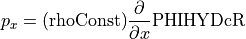
If you expand the “Data variables” section in the above Dataset summary, you’ll see a number of grid parameters, and you can look at their descriptions by clicking on the “sheet of paper” icon to the right of each one. To compute - and -derivatives of pressure, we recall that the pressure variable (PHIHYD) is located on coordinates (time,k,tile,j,i). The (j,i) coordinates indicate that pressure is “centered” in a given grid cell. The distance between the centers of grid cells is given by the variables dxC and dyC (the “C” indicates distance between grid cell centers).
Now we can compute the derivatives of pressure and the right-hand side of the geostrophic balance equations. Because the native grid of ECCOv4 is composed of 13 tiles, when we difference or interpolate values across the tile edges, things can get complicated! Fortunately the xgcm
package that was imported previously can help us with those operations. First we specify the connections between tiles in a Python dictionary, then create an xgcm Grid object that will allow us to carry out
differencing and interpolation across the tile edges. We will need to both difference and interpolate to end up with pressure gradient values that are located at the center (i,j) of the grid cells.
[16]:
# # create xgcm Grid object
xgcm_grid = ecco.get_llc_grid(ds_grid)
# compute derivatives of pressure in x and y
d_press_dx = (xgcm_grid.diff(rhoConst*pressanom,axis="X",boundary='extend'))/ds_grid.dxC
d_press_dy = (xgcm_grid.diff(rhoConst*pressanom,axis="Y",boundary='extend'))/ds_grid.dyC
# convert DataArray content from dask to numpy arrays
# (dask arrays might have issues with interp_2d_vector fcn)
d_press_dx.data = d_press_dx.values
d_press_dy.data = d_press_dy.values
# interpolate (vector) gradient values to center of grid cells
import warnings
with warnings.catch_warnings():
warnings.simplefilter("ignore") # use this to ignore future warnings caused by interp_2d_vector function
press_grads_interp = xgcm_grid.interp_2d_vector({"X":d_press_dx,"Y":d_press_dy},boundary='extend')
dp_dx = press_grads_interp['X']
dp_dy = press_grads_interp['Y']
dp_dx.name = 'dp_dx'
dp_dy.name = 'dp_dy'
dp_dx
[16]:
<xarray.DataArray 'dp_dx' (time: 1, k: 50, tile: 13, j: 90, i: 90)> array([[[[[ nan, nan, nan, ..., nan, nan, nan], [ nan, nan, nan, ..., nan, nan, nan], [ nan, nan, nan, ..., nan, nan, nan], ..., [-1.78578217e-03, -2.80201435e-04, 4.48737061e-04, ..., 2.56811129e-03, 2.54054624e-03, 2.38151103e-03], [-1.97579130e-03, -1.17824820e-04, 6.02442888e-04, ..., 2.95511540e-03, 3.09964363e-03, 3.09713813e-03], [-1.60034164e-03, 3.31102929e-04, 6.47389097e-04, ..., 3.22869234e-03, 3.55401146e-03, 3.75702744e-03]], [[-8.98729253e-04, 7.29348627e-04, 2.39784946e-04, ..., 3.42662539e-03, 3.89235793e-03, 4.29460499e-03], [-2.40144931e-04, 7.03949365e-04, -7.84797710e-04, ..., 3.54899094e-03, 4.10596048e-03, 4.68219491e-03], [ 5.17581939e-05, 1.75516907e-04, -2.09984998e-03, ..., 3.58781964e-03, 4.15722188e-03, 4.85306140e-03], ... nan, nan, nan], [ nan, nan, nan, ..., nan, nan, nan], [ nan, nan, nan, ..., nan, nan, nan]], [[ nan, nan, nan, ..., nan, nan, nan], [ nan, nan, nan, ..., nan, nan, nan], [ nan, nan, nan, ..., nan, nan, nan], ..., [ nan, nan, nan, ..., nan, nan, nan], [ nan, nan, nan, ..., nan, nan, nan], [ nan, nan, nan, ..., nan, nan, nan]]]]], dtype=float32) Coordinates: * i (i) int32 0 1 2 3 4 5 6 7 8 9 10 ... 80 81 82 83 84 85 86 87 88 89 * j (j) int32 0 1 2 3 4 5 6 7 8 9 10 ... 80 81 82 83 84 85 86 87 88 89 * k (k) int32 0 1 2 3 4 5 6 7 8 9 10 ... 40 41 42 43 44 45 46 47 48 49 * tile (tile) int32 0 1 2 3 4 5 6 7 8 9 10 11 12 Dimensions without coordinates: time
- time: 1
- k: 50
- tile: 13
- j: 90
- i: 90
- nan nan nan nan nan nan nan nan ... nan nan nan nan nan nan nan nan
array([[[[[ nan, nan, nan, ..., nan, nan, nan], [ nan, nan, nan, ..., nan, nan, nan], [ nan, nan, nan, ..., nan, nan, nan], ..., [-1.78578217e-03, -2.80201435e-04, 4.48737061e-04, ..., 2.56811129e-03, 2.54054624e-03, 2.38151103e-03], [-1.97579130e-03, -1.17824820e-04, 6.02442888e-04, ..., 2.95511540e-03, 3.09964363e-03, 3.09713813e-03], [-1.60034164e-03, 3.31102929e-04, 6.47389097e-04, ..., 3.22869234e-03, 3.55401146e-03, 3.75702744e-03]], [[-8.98729253e-04, 7.29348627e-04, 2.39784946e-04, ..., 3.42662539e-03, 3.89235793e-03, 4.29460499e-03], [-2.40144931e-04, 7.03949365e-04, -7.84797710e-04, ..., 3.54899094e-03, 4.10596048e-03, 4.68219491e-03], [ 5.17581939e-05, 1.75516907e-04, -2.09984998e-03, ..., 3.58781964e-03, 4.15722188e-03, 4.85306140e-03], ... nan, nan, nan], [ nan, nan, nan, ..., nan, nan, nan], [ nan, nan, nan, ..., nan, nan, nan]], [[ nan, nan, nan, ..., nan, nan, nan], [ nan, nan, nan, ..., nan, nan, nan], [ nan, nan, nan, ..., nan, nan, nan], ..., [ nan, nan, nan, ..., nan, nan, nan], [ nan, nan, nan, ..., nan, nan, nan], [ nan, nan, nan, ..., nan, nan, nan]]]]], dtype=float32)
- i(i)int320 1 2 3 4 5 6 ... 84 85 86 87 88 89
- axis :
- X
- long_name :
- grid index in x for variables at tracer and 'v' locations
- swap_dim :
- XC
- comment :
- In the Arakawa C-grid system, tracer (e.g., THETA) and 'v' variables (e.g., VVEL) have the same x coordinate on the model grid.
- coverage_content_type :
- coordinate
array([ 0, 1, 2, 3, 4, 5, 6, 7, 8, 9, 10, 11, 12, 13, 14, 15, 16, 17, 18, 19, 20, 21, 22, 23, 24, 25, 26, 27, 28, 29, 30, 31, 32, 33, 34, 35, 36, 37, 38, 39, 40, 41, 42, 43, 44, 45, 46, 47, 48, 49, 50, 51, 52, 53, 54, 55, 56, 57, 58, 59, 60, 61, 62, 63, 64, 65, 66, 67, 68, 69, 70, 71, 72, 73, 74, 75, 76, 77, 78, 79, 80, 81, 82, 83, 84, 85, 86, 87, 88, 89])
- j(j)int320 1 2 3 4 5 6 ... 84 85 86 87 88 89
- axis :
- Y
- long_name :
- grid index in y for variables at tracer and 'u' locations
- swap_dim :
- YC
- comment :
- In the Arakawa C-grid system, tracer (e.g., THETA) and 'u' variables (e.g., UVEL) have the same y coordinate on the model grid.
- coverage_content_type :
- coordinate
array([ 0, 1, 2, 3, 4, 5, 6, 7, 8, 9, 10, 11, 12, 13, 14, 15, 16, 17, 18, 19, 20, 21, 22, 23, 24, 25, 26, 27, 28, 29, 30, 31, 32, 33, 34, 35, 36, 37, 38, 39, 40, 41, 42, 43, 44, 45, 46, 47, 48, 49, 50, 51, 52, 53, 54, 55, 56, 57, 58, 59, 60, 61, 62, 63, 64, 65, 66, 67, 68, 69, 70, 71, 72, 73, 74, 75, 76, 77, 78, 79, 80, 81, 82, 83, 84, 85, 86, 87, 88, 89])
- k(k)int320 1 2 3 4 5 6 ... 44 45 46 47 48 49
- axis :
- Z
- long_name :
- grid index in z for tracer variables
- swap_dim :
- Z
- coverage_content_type :
- coordinate
array([ 0, 1, 2, 3, 4, 5, 6, 7, 8, 9, 10, 11, 12, 13, 14, 15, 16, 17, 18, 19, 20, 21, 22, 23, 24, 25, 26, 27, 28, 29, 30, 31, 32, 33, 34, 35, 36, 37, 38, 39, 40, 41, 42, 43, 44, 45, 46, 47, 48, 49])
- tile(tile)int320 1 2 3 4 5 6 7 8 9 10 11 12
- long_name :
- lat-lon-cap tile index
- comment :
- The ECCO V4 horizontal model grid is divided into 13 tiles of 90x90 cells for convenience.
- coverage_content_type :
- coordinate
array([ 0, 1, 2, 3, 4, 5, 6, 7, 8, 9, 10, 11, 12])
Notice that the DataArray dp_dx has (j,i) horizontal coordinates, indicating that it is centered in the grid cells (after the interpolation operation). You can check that the same is true of dp_dy.
Right-hand side
Now we use density to compute and plot the right-hand side of the geostrophic balance equations. Note that these plots adjust the colormap in order to mask land areas in black.
[17]:
# compute right-hand side of geostrophic balance equations
geos_bal_RHS_1 = dp_dx/dens
geos_bal_RHS_2 = -dp_dy/dens
geos_bal_RHS_1 = geos_bal_RHS_1.where(ds_grid.maskC,np.nan) # mask land areas with NaNs
geos_bal_RHS_2 = geos_bal_RHS_2.where(ds_grid.maskC) # note that 'where' also masks with NaNs by default
# plot RHS of 1st geostrophic balance equation
curr_plot = (geos_bal_RHS_1.isel(tile=1,k=20)).plot(cmap='bwr')
# render NaNs (land areas) as black
cmap_nanmasked = curr_plot.cmap.copy()
cmap_nanmasked.set_bad('black')
curr_plot.cmap = cmap_nanmasked
# Note: Matplotlib plot text (such as the title below) can include LaTeX,
# but special characters such as backslash \ must include an extra "escape" backslash \
# in order to render correctly
plt.title('$(1/\\rho)p_x$')
# adjust colormap limits (multiply by 0.3)
curr_clim = np.asarray(curr_plot.get_clim())
curr_plot.set_clim(0.3*curr_clim)
plt.show()
Left-hand side
To compute the left-hand side of the geostrophic balance equations we need to center the velocity fields in the grid cells and compute . With the tools we’ve covered so far, this is fairly straightforward.
The code below also includes a function to scale the colormaps/colorbars based on the range of values present in the maps. As you write more code in Python, you will likely find yourself relying more and more on functions, rather than scripts or code blocks that run linearly top to bottom.
[18]:
"""
Note: the model velocities UVEL/u and VVEL/v are defined on the model grid axes.
On some tiles (like tile=1 which we plot below)
u and v will be essentially the eastward and northward velocity respectively.
But on other tiles the model axes are very different from geographic axes.
What matters for now is that these two components are always locally perpendicular.
"""
# interpolate velocities to center of grid cells
ds_vel_mo.UVEL.data = ds_vel_mo.UVEL.values
ds_vel_mo.VVEL.data = ds_vel_mo.VVEL.values
import warnings
with warnings.catch_warnings():
warnings.simplefilter("ignore")
vel_interp = xgcm_grid.interp_2d_vector({'X':ds_vel_mo.UVEL,'Y':ds_vel_mo.VVEL},boundary='extend')
u = vel_interp['X']
v = vel_interp['Y']
# compute f from latitude of grid cell centers
lat = ds_grid.YC
Omega = (2*np.pi)/86164
lat_rad = (np.pi/180)*lat # convert latitude from degrees to radians
f = 2*Omega*np.sin(lat_rad)
# compute left-hand side of geostrophic balance equations
geos_bal_LHS_1 = f*v
geos_bal_LHS_2 = f*u
geos_bal_LHS_1 = geos_bal_LHS_1.where(ds_grid.maskC) # mask land areas with NaNs
geos_bal_LHS_2 = geos_bal_LHS_2.where(ds_grid.maskC)
# Introduce function to scale colormap
def cmap_zerocent_scale(plot,scale_factor):
"""
Center colormap at zero and scale relative to existing |maximum| value,
given plot object and scale_factor, a number of type float.
Returns new colormap limits as new_clim.
"""
curr_clim = plot.get_clim()
new_clim = (scale_factor*np.max(np.abs(curr_clim)))*np.array([-1,1])
plot.set_clim(new_clim)
return new_clim
# tile and k indices to plot
tile_plot = 1
k_plot = 20
# dictionary to select tile and k indices (can then pass this to isel to save space)
isel_dict = {'tile':tile_plot,'k':k_plot}
# create figure
fig,axs = plt.subplots(2,2,figsize=(11,8))
# set NaN masking in colormap in advance
# (in contrast to previous method setting NaN mask after plot is created)
seismic_nanmasked = plt.get_cmap('seismic').copy()
seismic_nanmasked.set_bad('black')
curr_ax = axs[0,0]
curr_plot = curr_ax.pcolormesh((geos_bal_LHS_1.isel(tile=tile_plot,k=k_plot)).squeeze(),cmap=seismic_nanmasked)
plot_clim = cmap_zerocent_scale(curr_plot,0.3) # centers colormap at zero and scales extent by 0.3
curr_ax.set_title('$fv$')
fig.colorbar(curr_plot,ax=curr_ax)
curr_ax = axs[0,1]
curr_plot = curr_ax.pcolormesh((geos_bal_RHS_1.isel(tile=tile_plot,k=k_plot)).squeeze(),cmap=seismic_nanmasked)
curr_plot.set_clim(plot_clim) # set RHS colormap limits to same values as LHS
curr_ax.set_title('$(1/\\rho)p_x$')
fig.colorbar(curr_plot,ax=curr_ax)
curr_ax = axs[1,0]
curr_plot = curr_ax.pcolormesh((geos_bal_LHS_2.isel(tile=tile_plot,k=k_plot)).squeeze(),cmap=seismic_nanmasked)
plot_clim = cmap_zerocent_scale(curr_plot,0.3)
curr_ax.set_title('$fu$')
fig.colorbar(curr_plot,ax=curr_ax)
curr_ax = axs[1,1]
curr_plot = curr_ax.pcolormesh((geos_bal_RHS_2.isel(tile=tile_plot,k=k_plot)).squeeze(),cmap=seismic_nanmasked)
curr_plot.set_clim(plot_clim) # set RHS colormap limits to same values as LHS
curr_ax.set_title('$-(1/\\rho)p_y$')
fig.colorbar(curr_plot,ax=curr_ax)
plt.show()
As you can see, the left and right plots in each row are nearly identical!
We can also plot the equation divided by so each side is in units of velocity. Actual velocities , are on the left, and geostrophic velocities , are on the right–the velocities that are “explained” by geostrophic balance.
[19]:
# compute geostrophic velocities
v_g = geos_bal_RHS_1/f
u_g = geos_bal_RHS_2/f
v_g = v_g.where(ds_grid.maskC) # mask land areas with NaNs
u_g = u_g.where(ds_grid.maskC)
# tile and k indices to plot
tile_plot = 1
k_plot = 20
# dictionary to select tile and k indices (can then pass this to isel to save space)
isel_dict = {'tile':tile_plot,'k':k_plot}
# identify depth level for plot titles
depth_plot_level = -ds_grid.Z[k_plot].values
# convert depth level (rounded to nearest meter) to a string for plot titles
depth_str = str(int(depth_plot_level))
# plot LHS and RHS of equations for tile = 1, k = 20 in a figure with 2x2 subplots
# arrays need to have singleton (time) dimension removed with .squeeze() before plotting
# create figure
fig,axs = plt.subplots(2,2,figsize=(11,8))
curr_ax = axs[0,0]
curr_plot = curr_ax.pcolormesh((v.isel(isel_dict)).squeeze(),cmap=seismic_nanmasked)
plot_clim = cmap_zerocent_scale(curr_plot,0.3)
curr_ax.set_title('$v$, ' + depth_str + ' m depth')
cbar = fig.colorbar(curr_plot,ax=axs[0,0])
# cbar.set_label('Velocity [m s$^{-1}$]')
curr_ax = axs[0,1]
curr_plot = curr_ax.pcolormesh((v_g.isel(isel_dict)).squeeze(),cmap=seismic_nanmasked)
curr_plot.set_clim(plot_clim)
curr_ax.set_title('$v_g$, ' + depth_str + ' m depth')
cbar = fig.colorbar(curr_plot,ax=axs[0,1])
cbar.set_label('Velocity [m s$^{-1}$]')
curr_ax = axs[1,0]
curr_plot = curr_ax.pcolormesh((u.isel(isel_dict)).squeeze(),cmap=seismic_nanmasked)
plot_clim = cmap_zerocent_scale(curr_plot,0.3)
curr_ax.set_title('$u$, ' + depth_str + ' m depth')
cbar = fig.colorbar(curr_plot,ax=axs[1,0])
# cbar.set_label('Velocity [m s$^{-1}$]')
curr_ax = axs[1,1]
curr_plot = axs[1,1].pcolormesh((u_g.isel(isel_dict)).squeeze(),cmap=seismic_nanmasked)
curr_plot.set_clim(plot_clim)
curr_ax.set_title('$u_g$, ' + depth_str + ' m depth')
cbar = fig.colorbar(curr_plot,ax=axs[1,1])
cbar.set_label('Velocity [m s$^{-1}$]')
plt.show()
Notice some weirdness in the geostrophic velocity maps (right column) near the equator. Hmm, why would that be…?
We can also visualize (actual) velocities as vectors relative to pressure anomaly contours. This looks much like maps of the atmospheric circulation that you might see in a weather report.
[20]:
pressanom_plot = pressanom.where(ds_grid.maskC) # mask land areas with NaNs
# tile and k indices to plot
tile_plot = 1
k_plot = 20
# dictionary to select tile and k indices (can then pass this to isel to save space)
isel_dict = {'tile':tile_plot,'k':k_plot}
# identify depth level for plot titles
depth_plot_level = -ds_grid.Z[k_plot].values
# convert depth level (rounded to nearest meter) to a string for plot titles
depth_str = str(int(depth_plot_level))
fig,ax = plt.subplots(figsize=(10,8))
# create 'bwr' colormap with NaN masking
bwr_nanmasked = plt.get_cmap('bwr').copy()
bwr_nanmasked.set_bad('black')
# plot filled contours, contour lines, and land mask
# (plots with higher zorder values are visible over lower zorder values)
curr_plot = (pressanom_plot.isel(isel_dict).squeeze()).plot.contourf(cmap=bwr_nanmasked,levels=29,vmin=86,vmax=100,zorder=50)
curr_contours = (pressanom_plot.isel(isel_dict).squeeze()).plot.contour(colors='black',levels=29,vmin=86,vmax=100,alpha=0.5,\
linewidths=0.5,zorder=100)
curr_plot_mask = (pressanom_plot.isel(isel_dict).squeeze()).plot(cmap=bwr_nanmasked,add_colorbar=False,vmin=86,vmax=100,zorder=0)
# plot velocity vectors using quiver
u_plot = (u.isel(isel_dict)).squeeze()
v_plot = (v.isel(isel_dict)).squeeze()
arrow_spacing = 3 # plot arrows spaced out (otherwise there is an arrow for every grid point)
ind_arrow_plot = np.r_[1:u_plot.shape[-1]:arrow_spacing]
curr_velplot = ax.quiver(ind_arrow_plot,ind_arrow_plot,u_plot[ind_arrow_plot,ind_arrow_plot],\
v_plot[ind_arrow_plot,ind_arrow_plot],scale=1.5,zorder=150)
ax.set_title('Pressure anomaly (shading) and velocity (arrows), ' + depth_str + ' m depth')
plt.show()
Assessment of geostrophic balance
Normalized difference maps
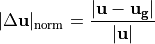
How can we can assess the variation in geostrophic balance and how well it accounts for ocean velocity globally? One way is to plot the normalized difference between actual and geostrophic velocities. We could do this for and components separately, but to get the most information in one plot, we can do this with the magnitude of difference between the velocity vectors.
[21]:
# difference between actual and geostrophic velocity vectors (in complex plane)
u_diff = u - u_g
v_diff = v - v_g
vel_diff_complex = u_diff + (1j*v_diff) # in Python, imaginary number i is indicated by 1j
vel_complex = u + (1j*v)
# normalize magnitude of difference vector by magnitude of actual velocity
vel_diff_abs = np.abs(vel_diff_complex)
vel_abs = np.abs(vel_complex)
vel_diff_norm = vel_diff_abs/vel_abs
# tile and k indices to plot
tile_plot = 1
k_plot = 20
# dictionary to select tile and k indices (can then pass this to isel to save space)
isel_dict = {'tile':tile_plot,'k':k_plot}
# identify depth level for plot titles
depth_plot_level = -ds_grid.Z[k_plot].values
# convert depth level (rounded to nearest meter) to a string for plot titles
depth_str = str(int(depth_plot_level))
# plot normalized difference
fig,ax = plt.subplots(figsize=(10,8))
array_plot = (vel_diff_norm.isel(isel_dict)).squeeze()
# let's use a logarithmic color scale for this plot!
import matplotlib.colors as colors
# set axis limits to 0.01 and 1 (values outside this range will be saturated)
curr_plot = ax.pcolormesh(array_plot,norm=colors.LogNorm(vmin=0.01,vmax=1),cmap=seismic_nanmasked)
fig.colorbar(curr_plot,ax=ax)
ax.set_title('|Delta u|_norm, actual vs. geostrophic velocity,' + depth_str + ' m depth')
plt.show()
A normalized difference of 0.1 (white on the above map) can be considered an approximate threshold for where the geostrophic velocity is a decent predictor of actual velocity. Therefore, what the above map shows is areas where geostrophic velocity is a good predictor of actual velocity (blue), and areas where the geostrophic velocity is a poor predictor (red). Note that where the actual velocity magnitude is very small, the map may show red even though the velocity difference itself isn’t large. To focus on areas with more substantial velocities, we can remap with the small-velocity points masked out.
To help us out with this, we’ll introduce a new function that plots a mask. Note that we can also use this function (instead of masking with set_bad
) to mask land areas, and we’ll do this below.
[22]:
# Introduce function to plot mask as pcolormesh
def plot_mask(*args,ax=None,color):
"""
Plot mask, given input parameters:
- X, Y: (optional) coordinates as 1-D or 2-D NumPy arrays or xarray DataArrays
- mask: 2-D array of boolean values (True/False or 1/0), NumPy or xarray
- axes: axes to plot on, defaults to current axes
- color: a string indicating a color in Matplotlib, or a 3-element tuple or NumPy array indicating RGB color values
Returns plot_obj, the plot object of the mask
"""
if len(args) == 1:
mask = args[0]
else:
X = args[0]
Y = args[1]
mask = args[2]
# set alpha values to 1 where mask is plotted, 0 otherwise
if str(type(mask))[0:5] == 'xarray':
mask = mask.values
# get color for mask
if isinstance(color,str):
import matplotlib.colors as mcolors
color_rgb = mcolors.to_rgb(color)
elif (isinstance(color,tuple)) and (len(color) == 3):
color_rgb = np.asarray(color)
elif (isinstance(color,np.ndarray)) and (len(color) == 3):
color_rgb = color
else:
raise TypeError("input parameter 'color' has incorrect type or number of elements")
# create a colormap using a 2x4 array with two RGBA entries
# the RGB entries are the same in each row
# in the 1st row alpha=0, in the 2nd row alpha=1
cmap_array = np.hstack((np.tile(color_rgb,(2,1)),np.array([[0],[1]])))
from matplotlib.colors import ListedColormap
colormap = ListedColormap(cmap_array)
# get axis limits of existing plot
if ax is None:
ax = plt.gca()
existing_xlim = ax.get_xlim()
existing_ylim = ax.get_ylim()
# plot mask using colormap just created, with alpha=1 where mask=1 or True
if len(args) == 1:
plot_obj = ax.pcolormesh(mask,cmap=colormap,vmin=0.,vmax=1.,zorder=50)
else:
plot_obj = ax.pcolormesh(X,Y,mask,cmap=colormap,vmin=0.,vmax=1.,zorder=50)
# set axis limits of mask to axis limits of existing plot
ax.set_xlim(existing_xlim)
ax.set_ylim(existing_ylim)
return plot_obj
Now we’ll create two plots side-by-side, one without and one with the small-velocity mask.
[23]:
# load land mask (a boolean array) from grid parameters
# Note: maskC has True (1) over water and False (0) over land
# we want the reverse for a land_mask, so ~ switches the boolean values
land_mask = ~ds_grid.maskC
# small velocity mask
mask_threshold = 0.005 # mask out velocities <0.5 cm s-1
# Note: the .values attribute contains the content of the data variable as a NumPy array.
# This allows additional operations not permitted in xarray,
# such as boolean indexing used here to mask with NaNs.
mask_smallvel = (vel_abs < mask_threshold)
# dictionary to select tile and k indices (can then pass this to isel to save space)
isel_dict = {'tile':tile_plot,'k':k_plot}
# plot normalized difference without and with mask
fig,axs = plt.subplots(1,2,figsize=(15,6))
curr_ax = axs[0]
curr_ax.tick_params(labelsize=14)
array_plot = vel_diff_norm.isel(isel_dict).squeeze()
curr_plot = curr_ax.pcolormesh(array_plot,norm=colors.LogNorm(vmin=0.01,vmax=1),cmap='seismic')
# plot land mask in black
plot_mask(land_mask.isel(isel_dict).squeeze(),ax=curr_ax,color='black')
curr_ax.set_title('|Delta u|_norm, actual vs. geostrophic velocity',fontsize=14)
fig.colorbar(curr_plot,ax=curr_ax)
curr_ax = axs[1]
curr_ax.tick_params(labelsize=14)
array_plot = vel_diff_norm.isel(isel_dict).squeeze()
curr_plot = curr_ax.pcolormesh(array_plot,norm=colors.LogNorm(vmin=0.01,vmax=1),cmap='seismic')
plot_mask(land_mask.isel(isel_dict).squeeze(),ax=curr_ax,color='black')
# plot small velocity mask in gray color, RGB=(0.5,0.5,0.5)
plot_mask(mask_smallvel.isel(isel_dict).squeeze(),ax=curr_ax,color=(0.5,0.5,0.5))
curr_ax.set_title('|Delta u|_norm, actual vs. geostrophic velocity, with mask',fontsize=14)
fig.colorbar(curr_plot,ax=curr_ax)
plt.show()
Global maps
Having mastered mapping on a single tile of the model grid, we can now plot maps that show the model’s entire horizontal global domain. We’ll use functions that are part of the ecco_v4_py
package to do this in two ways here: (1) plotting 13 tiles side-by-side, and (2) plotting the model fields regridded to a global lat-lon projection.
First the 13 tiles map. The Plotting Tiles tutorial shows a number of configurations that tiles can be plotted; here we use the latlon layout with the Arctic tile adjacent to tile=10.
[24]:
# k index (depth level) to plot
k_plot = 20
# identify depth level for plot titles
depth_plot_level = -ds_grid.Z[k_plot].values
# convert depth level (rounded to nearest meter) to a string for plot titles
depth_str = str(int(depth_plot_level))
# 13 tiles map using ecco_v4_py function plot_tiles
# (we'll leave out the small-velocity mask for the global maps)
curr_obj = ecco.plot_tiles(vel_diff_norm.isel(k=k_plot).squeeze(),\
cmap=seismic_nanmasked,show_colorbar=False,fig_size=10,\
layout='latlon',rotate_to_latlon=True,\
show_tile_labels=False,\
Arctic_cap_tile_location=10)
curr_fig = curr_obj[0]
# loop through tiles to adjust color scaling and add mask
tile_order = np.array([-1,-1,-1,6, \
2,5,7,10, \
1,4,8,11, \
0,3,9,12])
for idx,curr_ax in enumerate(curr_fig.get_axes()):
# set color scaling to lognormal range we used previously
if len(curr_ax.get_images()) > 0:
(curr_ax.get_images()[0]).norm = colors.LogNorm(vmin=0.01,vmax=1)
# add colorbar
cbar_ax = curr_fig.add_axes([0.95,0.2,0.025,0.6])
cbar = curr_fig.colorbar(plt.cm.ScalarMappable(\
norm=colors.LogNorm(vmin=0.01,vmax=1),\
cmap='seismic'),cax=cbar_ax)
# add title
curr_fig.suptitle('|Delta u|_norm, actual vs. geostrophic velocity, ' + depth_str + ' m depth')
plt.show()
And on a global map projection (here the Robinson projection is used):
[25]:
# k index (depth level) to plot
k_plot = 20
# global map projection using ecco_v4_py function plot_proj_to_latlon_grid
# Query help(ecco.plot_proj_to_latlon_grid) for a full list of input arguments.
curr_obj = ecco.plot_proj_to_latlon_grid(ds_grid.XC,ds_grid.YC,\
vel_diff_norm.isel(k=k_plot).squeeze(),\
cmap=seismic_nanmasked,show_colorbar=False,\
show_land=True,projection_type='robin',\
user_lon_0=-67,plot_type='pcolormesh')
curr_fig = curr_obj[0]
curr_ax = curr_obj[1]
curr_fig.set_figwidth(15)
curr_fig.set_figheight(10)
import matplotlib as mpl
# set color scaling to lognormal range
for handle in curr_ax.get_children():
if isinstance(handle,mpl.collections.QuadMesh):
handle.norm = colors.LogNorm(vmin=0.01,vmax=1)
# add colorbar with correct scaling
cbar_ax = curr_fig.add_axes([0.95,0.2,0.025,0.6])
cbar = curr_fig.colorbar(plt.cm.ScalarMappable(\
norm=colors.LogNorm(vmin=0.01,vmax=1),\
cmap=seismic_nanmasked),cax=cbar_ax)
# add title
curr_ax.set_title('|Delta u|_norm, actual vs. geostrophic velocity, ' + depth_str + ' m depth')
plt.show()
-179.875 112.875
-180.0 113.0
-89.875 89.875
-90.0 90.0
113.12547814606742 179.87453185393258
113.00001 180.0
-89.875 89.875
-90.0 90.0
Latitude and depth dependence
We can also plot along a transect to consider its variation with depth. Let’s plot an example along i=40
on tile=1
(which follows the line of longitude ):
[26]:
# tile and i indices to plot
tile_plot = 1
i_plot = 40
# dictionary to select tile and i (i_g) indices
isel_dict = {'tile':tile_plot,'i':i_plot}
isel_dict_ig = {'tile':tile_plot,'i_g':i_plot}
# compute land and small velocity masks
curr_land_mask = land_mask.isel(isel_dict).squeeze()
curr_mask_smallvel = mask_smallvel.isel(isel_dict).squeeze()
# plot normalized difference without and with mask
# here we'll plot top 25 and bottom 25 depth levels separately to accommodate different scales
fig,axs = plt.subplots(2,2,figsize=(15,10))
curr_ax = axs[0,0]
# Note: when specifying coordinates with a data array of size MxN
# Matplotlib will only use "flat" shading if coordinate dimensions are one larger than data array
# i.e., length M+1 and N+1, or (M+1)x(N+1), otherwise defaults to "nearest" shading
# bounding coordinates for upper pcolormesh plots
lat_plot = np.hstack(((ds_grid.YG.isel(isel_dict_ig)).squeeze(),\
ds_grid.YC_bnds.isel({**isel_dict,'j':-1,'nb':3})))
depth_plot = -ds_grid.Zp1[0:26].squeeze() # top 25 depth levels
array_plot = (vel_diff_norm.isel(isel_dict)).squeeze()
curr_plot = curr_ax.pcolormesh(lat_plot,depth_plot,array_plot[0:25,:],\
norm=colors.LogNorm(vmin=0.01,vmax=1),cmap='seismic')
plot_mask(lat_plot,depth_plot,curr_land_mask[0:25,:],ax=curr_ax,color='black')
curr_ax.set_ylim(curr_ax.get_ylim()[::-1])
curr_ax.set_ylabel('Depth [m]')
curr_ax.set_title('|Delta u|_norm, actual vs. geostrophic velocity',fontsize=14)
fig.colorbar(curr_plot,ax=curr_ax)
curr_ax = axs[0,1]
array_plot = (vel_diff_norm.isel(isel_dict)).squeeze()
curr_plot = curr_ax.pcolormesh(lat_plot,depth_plot,array_plot[0:25,:],\
norm=colors.LogNorm(vmin=0.01,vmax=1),cmap='seismic')
plot_mask(lat_plot,depth_plot,curr_land_mask[0:25,:],ax=curr_ax,color='black')
plot_mask(lat_plot,depth_plot,curr_mask_smallvel[0:25,:],ax=curr_ax,color=(0.5,0.5,0.5))
curr_ax.set_ylim(curr_ax.get_ylim()[::-1])
curr_ax.set_ylabel('Depth [m]')
curr_ax.set_title('|Delta u|_norm, actual vs. geostrophic velocity, with mask',fontsize=14)
fig.colorbar(curr_plot,ax=curr_ax)
curr_ax = axs[1,0]
# bounding coordinates for lower pcolormesh plots
lat_plot = np.hstack(((ds_grid.YG.isel(isel_dict_ig)).squeeze(),\
ds_grid.YC_bnds.isel({**isel_dict,'j':-1,'nb':3})))
depth_plot = -ds_grid.Zp1[25:].squeeze() # bottom 25 depth levels
array_plot = (vel_diff_norm.isel(isel_dict)).squeeze()
curr_plot = curr_ax.pcolormesh(lat_plot,depth_plot,array_plot[25:,:],\
norm=colors.LogNorm(vmin=0.01,vmax=1),cmap='seismic')
plot_mask(lat_plot,depth_plot,curr_land_mask[25:,:],ax=curr_ax,color='black')
curr_ax.set_ylim(curr_ax.get_ylim()[::-1])
curr_ax.set_ylabel('Depth [m]')
curr_ax.set_xlabel('Latitude')
fig.colorbar(curr_plot,ax=curr_ax)
curr_ax = axs[1,1]
array_plot = (vel_diff_norm.isel(isel_dict)).squeeze()
curr_plot = curr_ax.pcolormesh(lat_plot,depth_plot,array_plot[25:,:],\
norm=colors.LogNorm(vmin=0.01,vmax=1),cmap='seismic')
plot_mask(lat_plot,depth_plot,curr_land_mask[25:,:],ax=curr_ax,color='black')
plot_mask(lat_plot,depth_plot,curr_mask_smallvel[25:,:],ax=curr_ax,color=(0.5,0.5,0.5))
curr_ax.set_ylim(curr_ax.get_ylim()[::-1])
curr_ax.set_ylabel('Depth [m]')
curr_ax.set_xlabel('Latitude')
fig.colorbar(curr_plot,ax=curr_ax)
plt.show()
Can you see some patterns in the above plots? Most depths 100-1500 meters have a lot of blue, meaning geostrophic velocities are very good approximations of the actual velocities. But (1) close to the ocean surface, (2) close to the ocean bottom, and (3) near the equator there is a lot more red. So in those areas, some of the other terms in the momentum equations that we earlier considered to be negligible, may not actually be negligible. We’ll explore some of these other balances in upcoming tutorials.
For now, let’s explore these patterns in a more systematic way globally. The following code computes the normalized difference (weighted by the area of each grid cell) as a function of latitude and depth, for the global oceans. Note: the ``mean_weighted_binned`` function may take a few minutes to run over the global domain.
[27]:
# bins of latitude
lat_bin_spacing = 2
lat_bin_bounds = np.c_[-90:90:lat_bin_spacing] + np.array([[0,lat_bin_spacing]])
lat_bin_centers = np.mean(lat_bin_bounds,axis=-1)
# bins of depth
depth_bin_bounds = -ds_grid.Z_bnds.values
vel_diff_abs = np.abs(vel_diff_complex)
vel_abs = np.abs(vel_complex)
# function to loop through and compute weighted mean in bins
def mean_weighted_binned(value_field,weighting,bin_field,bin_bounds):
"""
Compute normalized difference in bins, given:
- value_field: field of values to average
- weighting: weighting of individual grid cells
- bin_field: field to use in binning
- bin_bounds: bound values of bins to use, as numpy array of size (N,2)
"""
mean_weighted_inbins = np.empty((bin_bounds.shape[0]))
mean_weighted_inbins.fill(np.nan)
bin_field_broadcast_flat = (np.ones(value_field.shape)*bin_field).flatten()
weighting_flat = weighting.flatten()
value_field_flat = value_field.flatten()
bin_idx_sorted = np.argsort(bin_field_broadcast_flat) # flatten and sort bin field values
sort_idx = (bin_field_broadcast_flat[bin_idx_sorted] >= bin_bounds[0,0]).nonzero()[0][0]
curr_idx = bin_idx_sorted[sort_idx]
curr_bin_val = bin_field_broadcast_flat[curr_idx]
curr_bin_num = ((bin_bounds[:,0] <= curr_bin_val) & (bin_bounds[:,1] > curr_bin_val)).nonzero()[0][0]
value_sum_inbin = 0.
weighting_sum_inbin = 0.
while curr_bin_val < bin_bounds[-1,1]:
if np.logical_and(~np.isnan(value_field_flat[curr_idx]),~np.isinf(value_field_flat[curr_idx])):
value_sum_inbin += weighting_flat[curr_idx]*value_field_flat[curr_idx]
weighting_sum_inbin += weighting_flat[curr_idx]
sort_idx += 1
if sort_idx >= len(bin_idx_sorted):
if weighting_sum_inbin > 0:
mean_weighted_inbins[curr_bin_num] = value_sum_inbin/weighting_sum_inbin
break
curr_idx = bin_idx_sorted[sort_idx]
curr_bin_val = bin_field_broadcast_flat[curr_idx]
if curr_bin_val >= bin_bounds[curr_bin_num,1]:
if weighting_sum_inbin > 0:
mean_weighted_inbins[curr_bin_num] = value_sum_inbin/weighting_sum_inbin
curr_bin_num = ((bin_bounds[:,0] <= curr_bin_val) & (bin_bounds[:,1] > curr_bin_val)).nonzero()[0][0]
value_sum_inbin = 0.
weighting_sum_inbin = 0.
return mean_weighted_inbins
# compute norm diff, weighting by horizontal area of grid cells and masks
curr_weighting = ((~mask_smallvel)*(ds_grid.maskC)*(ds_grid.rA)).values
diff_norm_lat = mean_weighted_binned(vel_diff_norm.values,curr_weighting,\
ds_grid.YC.values,lat_bin_bounds)
diff_norm_depth = mean_weighted_binned(vel_diff_norm.values,curr_weighting,\
np.expand_dims(-ds_grid.Z.values,axis=(-3,-2,-1)),\
depth_bin_bounds)
[28]:
# plot normalized difference, binned by latitude and by depth
fig,axs = plt.subplots(1,2,figsize=(15,8))
curr_ax = axs[0]
curr_ax.plot(lat_bin_centers,diff_norm_lat)
curr_ax.set_ylim(0.01,1)
curr_ax.set_yscale('log')
curr_ax.axhline(y=0.1,color='black',lw=2)
curr_ax.axvline(x=0,color='black',lw=1)
curr_ax.set_xlabel('Latitude')
curr_ax.set_ylabel('Normalized diff')
curr_ax.set_title('Normalized diff variation with latitude')
curr_ax = axs[1]
curr_ax.plot(diff_norm_depth,-ds_grid.Z)
# Note: in older versions of Matplotlib
# may need to use linthreshy instead of linthresh
curr_ax.set_yscale('symlog',linthresh=100)
curr_ax.set_ylim(curr_ax.get_ylim()[::-1])
curr_ax.set_yticks([0,50,100,500,1000,5000])
curr_ax.set_yticklabels(['0','50','100','500','1000','5000'])
curr_ax.set_xlim(0.01,1)
curr_ax.set_xscale('log')
curr_ax.axvline(x=0.1,color='black',lw=2)
curr_ax.set_xlabel('Normalized diff')
curr_ax.set_ylabel('Depth [m]')
curr_ax.set_title('Normalized diff variation with depth')
plt.show()
Based on the normalized diff = 0.1 threshold discussed before, geostrophic balance doesn’t hold particularly well at any latitude, and only at depths 100-1000 m. But let’s try this again, masking for only 100-1000 m depths in the latitude plot, and only latitudes more than 5 degrees from the equator in the depth plot.
[29]:
# latitude and depth masks
# create depth array that will broadcast correctly across horizontal dimensions
depth_expand_dims = np.expand_dims(-ds_grid.Z,axis=(-3,-2,-1))
depth_mask = np.logical_and(depth_expand_dims > 100,\
depth_expand_dims < 1000)
lat_mask = np.expand_dims((np.abs(ds_grid.YC) > 5),axis=0)
# compute norm diff with additional masks
curr_weighting = (depth_mask*(~mask_smallvel)*(ds_grid.maskC)*(ds_grid.rA)).values
diff_norm_lat_moremask = mean_weighted_binned(vel_diff_norm.values,curr_weighting,\
ds_grid.YC.values,lat_bin_bounds)
curr_weighting = (lat_mask*(~mask_smallvel)*(ds_grid.maskC)*(ds_grid.rA)).values
diff_norm_depth_moremask = mean_weighted_binned(vel_diff_norm.values,curr_weighting,\
depth_expand_dims,depth_bin_bounds)
[30]:
# plot normalized difference, binned by latitude and by depth
fig,axs = plt.subplots(1,2,figsize=(15,8))
curr_ax = axs[0]
curr_ax.plot(lat_bin_centers,diff_norm_lat,color=(0.3,0.3,0.3),label='All depths')
curr_ax.plot(lat_bin_centers,diff_norm_lat_moremask,color='blue',label='100-1000 m depth')
curr_ax.set_ylim(0.01,1)
curr_ax.set_yscale('log')
curr_ax.axhline(y=0.1,color='black',lw=2)
curr_ax.axvline(x=0,color='black',lw=1)
curr_ax.set_xlabel('Latitude')
curr_ax.set_ylabel('Normalized diff')
curr_ax.set_title('Normalized diff variation with latitude')
curr_ax.legend()
curr_ax = axs[1]
curr_ax.plot(diff_norm_depth,-ds_grid.Z,color=(0.3,0.3,0.3),label='All latitudes')
curr_ax.plot(diff_norm_depth_moremask,-ds_grid.Z,color='blue',label='>5 deg from equator')
# Note: in older versions of Matplotlib
# may need to use linthreshy instead of linthresh
curr_ax.set_yscale('symlog',linthresh=100)
curr_ax.set_ylim(curr_ax.get_ylim()[::-1])
curr_ax.set_yticks([0,50,100,500,1000,5000])
curr_ax.set_yticklabels(['0','50','100','500','1000','5000'])
curr_ax.set_xlim(0.01,1)
curr_ax.set_xscale('log')
curr_ax.axvline(x=0.1,color='black',lw=2)
curr_ax.set_xlabel('Normalized diff')
curr_ax.set_ylabel('Depth [m]')
curr_ax.set_title('Normalized diff variation with depth')
curr_ax.legend()
plt.show()
From the above plots, we can see that for areas in the 100-1000 m depth range, more than 5 degrees from the equator and in low-to-mid latitudes, velocities are overwhelmingly geostrophic. Outside of these areas, geostrophy is less predictive of velocity. The bin-averaged normalized differences show the loss of geostrophic balance at the equator, near the ocean surface, and in the deep ocean.
Before we finish, you can use the code below to save the binned normalized differences plotted above. This will be useful in the next tutorial.
[31]:
# save norm diff bin-averaged values (in numpy .npz format) for future use
diff_norm_inbins_filename = "diff_norm_geostr_bal.npz"
np.savez(diff_norm_inbins_filename,lat_bin_bounds=lat_bin_bounds,\
diff_norm_lat=diff_norm_lat,\
diff_norm_lat_moremask=diff_norm_lat_moremask,\
depth_bin_bounds=depth_bin_bounds,\
diff_norm_depth=diff_norm_depth,\
diff_norm_depth_moremask=diff_norm_depth_moremask)
Exercises
Having made it to the end of the tutorial, you’re now ready to try tweaking some of the code above to explore the ECCO data on your own. Here are a couple of suggested exercises, or you can develop your own ideas!
All of the mapping we just did was with monthly data for January 2000, but we also downloaded daily files for 1999-12-31 and 2000-01-01. Repeat the calculations and plots that we did, but this time with the daily files for one of those dates. How does geostrophic balance on daily timescales compare with monthly timescales? Why might they be different?
You probably noticed that geostrophic balance does not seem to be as good of an approximation for the flow in the Arctic as in other ocean basins. Focus on the monthly data in the Arctic tile (
tile=6
). Where is geostrophic balance the least effective, after masking out the smallest velocities? You’ll probably need to change a few parameters to get informative plots in this region of lower velocities. Pick a grid cell (i,j) where there are high normalized differences (preferably one where the ocean is >500 m deep), and make a plot comparing the depth profiles of geostrophic and actual u and v. For extra credit, also plot the depth profile of the angle of difference between the geostrophic and actual velocity vectors.
Tip: make a copy of this notebook before you edit it, so that you can try your own innovations while being able to easily return to the original notebook for comparison.
ecco_po_tutorials module
There are some functions used in this tutorial that it will be helpful to have access to for future tutorials (or your own analysis with ECCOv4). Hence these functions have been put into a ecco_po_tutorials module (a Python file) that will be imported in future tutorials. This module also includes a function to compute geostrophic velocities quickly, given the file containing density and pressure anomalies.
I recommend downloading it to the same directory where your tutorials are located. Some functions from this module may also be incorporated into the ecco_v4_py
package in the future.
References
Gill, A.E. (1982). Atmosphere-Ocean Dynamics. Academic Press, Elsevier.
Kundu, P.K. and Cohen, I.M. (2008). Fluid Mechanics (4th ed.). Elsevier.
Vallis, G.K. (2006). Atmospheric and Oceanic Fluid Dynamics. Cambridge University Press.