Loading the ECCOv4 state estimate fields on the native model grid

Objectives

Introduce several methods for opening and loading the ECCOv4 state estimate files on the native model grid.

Introduction

ECCOv4 native-grid state estimate fields are packaged together as NetCDF files. The ECCOv4 release 4 output files are available from PO.DAAC Cloud via NASA Earthdata. You can use the ecco_access Python package to access ECCOv4r4 datasets, either by specifying the dataset ShortName or querying the ECCO variable lists to identify the dataset(s) that you need.

For this tutorial, you will need the grid file used in the previous tutorial, and the monthly mean SSH, OBP, and temperature/salinity datasets from 2010-2012. The ShortNames for these datasets are ECCO_L4_SSH_LLC0090GRID_MONTHLY_V4R4, ECCO_L4_OBP_LLC0090GRID_MONTHLY_V4R4, and ECCO_L4_TEMP_SALINITY_LLC0090GRID_MONTHLY_V4R4.

NetCDF File Format

As of March 2023, ECCOv4 release 4 state estimate fields are distributed through PO.DAAC/ NASA Earthdata Cloud, and are stored as NetCDF files, with each file containing one granule. Most datasets contain a few related fields, and a granule is a dataset entry at a single time entry: a monthly mean, daily mean, or a snapshot at 0Z on a given day.

Typical file sizes in the LLC90 grid depend on how many fields are contained in a given dataset:

3D fields:  17-62 MB (2-8 fields x 1 time  x 50 levels x 13 tiles x 90 j x 90 i)
2D fields:  5-7 MB  (1-12 fields x 1 time  x  1 level  x 13 tiles x 90 j x 90 i)

Notice that there is a not a very large difference in the range of 2D file sizes between a granule of a dataset having 1 field (5 MB) and another dataset having 12 fields (7 MB). This is because most of the space in individual 2D files is occupied by grid parameters. One nice feature of using the xarray and Dask libraries is that we do not have to load the entire file contents into RAM to work with them. The glob and xarray libraries can also be used together to load multiple files (times) into your workspace as a single dataset, concatenating the data fields without repeating the grid parameters.

Open/view one ECCOv4 NetCDF file

In ECCO NetCDF files, all 13 tiles for a given year are aggregated into a single file. Therefore, we can use the open_dataset routine from xarray to open a single NetCDF variable file.

First set up the environment, load model grid parameters.

import numpy as np
import xarray as xr
from os.path import join,expanduser
import sys
import matplotlib.pyplot as plt
%matplotlib inline

import ecco_v4_py as ecco
import ecco_access as ea


# are you working in the AWS Cloud?
incloud_access = False

# indicate mode of access
# options are:
# 'download': direct download from internet to your local machine
# 'download_ifspace': like download, but only proceeds
#                     if your machine have sufficient storage
# 's3_open': access datasets in-cloud from an AWS instance
# 's3_open_fsspec': use jsons generated with fsspec and
#                   kerchunk libraries to speed up in-cloud access
# 's3_get': direct download from S3 in-cloud to an AWS instance
# 's3_get_ifspace': like s3_get, but only proceeds if your instance
#                   has sufficient storage
user_home_dir = expanduser('~')
download_dir = join(user_home_dir,'Downloads','ECCO_V4r4_PODAAC')
if incloud_access:
    access_mode = 's3_open_fsspec'
    download_root_dir = None
    jsons_root_dir = join(user_home_dir,'MZZ')
else:
    access_mode = 'download_ifspace'
    download_root_dir = download_dir
    jsons_root_dir = None

## Access datasets needed for this tutorial

grid_shortname = "ECCO_L4_GEOMETRY_LLC0090GRID_V4R4"
SSH_monthly_shortname = "ECCO_L4_SSH_LLC0090GRID_MONTHLY_V4R4"


ShortNames_list = ["ECCO_L4_GEOMETRY_LLC0090GRID_V4R4",\
                   "ECCO_L4_SSH_LLC0090GRID_MONTHLY_V4R4",\
                   "ECCO_L4_OBP_LLC0090GRID_MONTHLY_V4R4",\
                   "ECCO_L4_TEMP_SALINITY_LLC0090GRID_MONTHLY_V4R4"]

# ecco_podaac_access generates a dictionary whose keys are ShortNames, and whose values
# are a file path or list of file paths that can be passed to xr.open_dataset or xr.open_mfdataset
files_dict = ea.ecco_podaac_access(ShortNames_list,\
                                      StartDate='2010-01',EndDate='2012-12',\
                                      mode=access_mode,\
                                      download_root_dir=download_root_dir,\
                                      jsons_root_dir=jsons_root_dir,\
                                      max_avail_frac=0.5)

## load the grid
grid = xr.open_dataset(files_dict[ShortNames_list[0]])

Open a single ECCOv4 variable NetCDF file using open_dataset

SSH_dataset = xr.open_dataset(files_dict[ShortNames_list[1]])

SSH_dataset

<xarray.Dataset> Size: 7MB
Dimensions:    (i: 90, i_g: 90, j: 90, j_g: 90, tile: 13, time: 1, nv: 2, nb: 4)
Coordinates: (12/13)
  * i          (i) int32 360B 0 1 2 3 4 5 6 7 8 9 ... 81 82 83 84 85 86 87 88 89
  * i_g        (i_g) int32 360B 0 1 2 3 4 5 6 7 8 ... 81 82 83 84 85 86 87 88 89
  * j          (j) int32 360B 0 1 2 3 4 5 6 7 8 9 ... 81 82 83 84 85 86 87 88 89
  * j_g        (j_g) int32 360B 0 1 2 3 4 5 6 7 8 ... 81 82 83 84 85 86 87 88 89
  * tile       (tile) int32 52B 0 1 2 3 4 5 6 7 8 9 10 11 12
  * time       (time) datetime64[ns] 8B 2010-01-16T12:00:00
    ...         ...
    YC         (tile, j, i) float32 421kB ...
    XG         (tile, j_g, i_g) float32 421kB ...
    YG         (tile, j_g, i_g) float32 421kB ...
    time_bnds  (time, nv) datetime64[ns] 16B ...
    XC_bnds    (tile, j, i, nb) float32 2MB ...
    YC_bnds    (tile, j, i, nb) float32 2MB ...
Dimensions without coordinates: nv, nb
Data variables:
    SSH        (time, tile, j, i) float32 421kB ...
    SSHIBC     (time, tile, j, i) float32 421kB ...
    SSHNOIBC   (time, tile, j, i) float32 421kB ...
    ETAN       (time, tile, j, i) float32 421kB ...
Attributes: (12/57)
    acknowledgement:              This research was carried out by the Jet Pr...
    author:                       Ian Fenty and Ou Wang
    cdm_data_type:                Grid
    comment:                      Fields provided on the curvilinear lat-lon-...
    Conventions:                  CF-1.8, ACDD-1.3
    coordinates_comment:          Note: the global 'coordinates' attribute de...
    ...                           ...
    time_coverage_duration:       P1M
    time_coverage_end:            2010-02-01T00:00:00
    time_coverage_resolution:     P1M
    time_coverage_start:          2010-01-01T00:00:00
    title:                        ECCO Sea Surface Height - Monthly Mean llc9...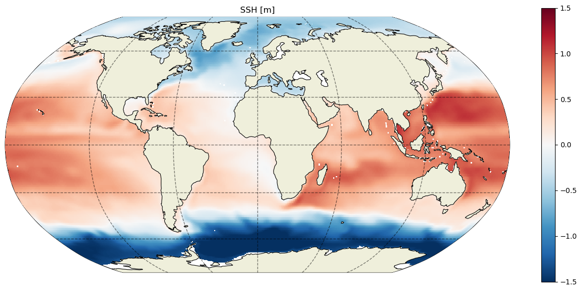
    uuid:                         9ce7afa6-400c-11eb-ab45-0cc47a3f49c3

xarray.Dataset

• Dimensions:
  • i: 90
  • i_g: 90
  • j: 90
  • j_g: 90
  • tile: 13
  • time: 1
  • nv: 2
  • nb: 4
• Coordinates: (13)
  • i
    (i)
    int32
    0 1 2 3 4 5 6 ... 84 85 86 87 88 89

    axis :

    X

    long_name :

    grid index in x for variables at tracer and 'v' locations

    swap_dim :

    XC

    comment :

    In the Arakawa C-grid system, tracer (e.g., THETA) and 'v' variables (e.g., VVEL) have the same x coordinate on the model grid.

    coverage_content_type :

    coordinate

    array([ 0,  1,  2,  3,  4,  5,  6,  7,  8,  9, 10, 11, 12, 13, 14, 15, 16, 17,
           18, 19, 20, 21, 22, 23, 24, 25, 26, 27, 28, 29, 30, 31, 32, 33, 34, 35,
           36, 37, 38, 39, 40, 41, 42, 43, 44, 45, 46, 47, 48, 49, 50, 51, 52, 53,
           54, 55, 56, 57, 58, 59, 60, 61, 62, 63, 64, 65, 66, 67, 68, 69, 70, 71,
           72, 73, 74, 75, 76, 77, 78, 79, 80, 81, 82, 83, 84, 85, 86, 87, 88, 89],
          dtype=int32)

  • i_g
    (i_g)
    int32
    0 1 2 3 4 5 6 ... 84 85 86 87 88 89

    axis :

    X

    long_name :

    grid index in x for variables at 'u' and 'g' locations

    c_grid_axis_shift :

    -0.5

    swap_dim :

    XG

    comment :

    In the Arakawa C-grid system, 'u' (e.g., UVEL) and 'g' variables (e.g., XG) have the same x coordinate on the model grid.

    coverage_content_type :

    coordinate

    array([ 0,  1,  2,  3,  4,  5,  6,  7,  8,  9, 10, 11, 12, 13, 14, 15, 16, 17,
           18, 19, 20, 21, 22, 23, 24, 25, 26, 27, 28, 29, 30, 31, 32, 33, 34, 35,
           36, 37, 38, 39, 40, 41, 42, 43, 44, 45, 46, 47, 48, 49, 50, 51, 52, 53,
           54, 55, 56, 57, 58, 59, 60, 61, 62, 63, 64, 65, 66, 67, 68, 69, 70, 71,
           72, 73, 74, 75, 76, 77, 78, 79, 80, 81, 82, 83, 84, 85, 86, 87, 88, 89],
          dtype=int32)

  • j
    (j)
    int32
    0 1 2 3 4 5 6 ... 84 85 86 87 88 89

    axis :

    Y

    long_name :

    grid index in y for variables at tracer and 'u' locations

    swap_dim :

    YC

    comment :

    In the Arakawa C-grid system, tracer (e.g., THETA) and 'u' variables (e.g., UVEL) have the same y coordinate on the model grid.

    coverage_content_type :

    coordinate

    array([ 0,  1,  2,  3,  4,  5,  6,  7,  8,  9, 10, 11, 12, 13, 14, 15, 16, 17,
           18, 19, 20, 21, 22, 23, 24, 25, 26, 27, 28, 29, 30, 31, 32, 33, 34, 35,
           36, 37, 38, 39, 40, 41, 42, 43, 44, 45, 46, 47, 48, 49, 50, 51, 52, 53,
           54, 55, 56, 57, 58, 59, 60, 61, 62, 63, 64, 65, 66, 67, 68, 69, 70, 71,
           72, 73, 74, 75, 76, 77, 78, 79, 80, 81, 82, 83, 84, 85, 86, 87, 88, 89],
          dtype=int32)

  • j_g
    (j_g)
    int32
    0 1 2 3 4 5 6 ... 84 85 86 87 88 89

    axis :

    Y

    long_name :

    grid index in y for variables at 'v' and 'g' locations

    c_grid_axis_shift :

    -0.5

    swap_dim :

    YG

    comment :

    In the Arakawa C-grid system, 'v' (e.g., VVEL) and 'g' variables (e.g., XG) have the same y coordinate.

    coverage_content_type :

    coordinate

    array([ 0,  1,  2,  3,  4,  5,  6,  7,  8,  9, 10, 11, 12, 13, 14, 15, 16, 17,
           18, 19, 20, 21, 22, 23, 24, 25, 26, 27, 28, 29, 30, 31, 32, 33, 34, 35,
           36, 37, 38, 39, 40, 41, 42, 43, 44, 45, 46, 47, 48, 49, 50, 51, 52, 53,
           54, 55, 56, 57, 58, 59, 60, 61, 62, 63, 64, 65, 66, 67, 68, 69, 70, 71,
           72, 73, 74, 75, 76, 77, 78, 79, 80, 81, 82, 83, 84, 85, 86, 87, 88, 89],
          dtype=int32)

  • tile
    (tile)
    int32
    0 1 2 3 4 5 6 7 8 9 10 11 12

    long_name :

    lat-lon-cap tile index

    comment :

    The ECCO V4 horizontal model grid is divided into 13 tiles of 90x90 cells for convenience.

    coverage_content_type :

    coordinate

    array([ 0,  1,  2,  3,  4,  5,  6,  7,  8,  9, 10, 11, 12], dtype=int32)

  • time
    (time)
    datetime64[ns]
    2010-01-16T12:00:00

    long_name :

    center time of averaging period

    axis :

    T

    bounds :

    time_bnds

    coverage_content_type :

    coordinate

    standard_name :

    time

    array(['2010-01-16T12:00:00.000000000'], dtype='datetime64[ns]')

  • XC
    (tile, j, i)
    float32
    ...

    long_name :

    longitude of tracer grid cell center

    units :

    degrees_east

    coordinate :

    YC XC

    bounds :

    XC_bnds

    comment :

    nonuniform grid spacing

    coverage_content_type :

    coordinate

    standard_name :

    longitude

    [105300 values with dtype=float32]

  • YC
    (tile, j, i)
    float32
    ...

    long_name :

    latitude of tracer grid cell center

    units :

    degrees_north

    coordinate :

    YC XC

    bounds :

    YC_bnds

    comment :

    nonuniform grid spacing

    coverage_content_type :

    coordinate

    standard_name :

    latitude

    [105300 values with dtype=float32]

  • XG
    (tile, j_g, i_g)
    float32
    ...

    long_name :

    longitude of 'southwest' corner of tracer grid cell

    units :

    degrees_east

    coordinate :

    YG XG

    comment :

    Nonuniform grid spacing. Note: 'southwest' does not correspond to geographic orientation but is used for convenience to describe the computational grid. See MITgcm dcoumentation for details.

    coverage_content_type :

    coordinate

    standard_name :

    longitude

    [105300 values with dtype=float32]

  • YG
    (tile, j_g, i_g)
    float32
    ...

    long_name :

    latitude of 'southwest' corner of tracer grid cell

    units :

    degrees_north

    coordinate :

    YG XG

    comment :

    Nonuniform grid spacing. Note: 'southwest' does not correspond to geographic orientation but is used for convenience to describe the computational grid. See MITgcm dcoumentation for details.

    coverage_content_type :

    coordinate

    standard_name :

    latitude

    [105300 values with dtype=float32]

  • time_bnds
    (time, nv)
    datetime64[ns]
    ...

    comment :

    Start and end times of averaging period.

    coverage_content_type :

    coordinate

    long_name :

    time bounds of averaging period

    [2 values with dtype=datetime64[ns]]

  • XC_bnds
    (tile, j, i, nb)
    float32
    ...

    comment :

    Bounds array follows CF conventions. XC_bnds[i,j,0] = 'southwest' corner (j-1, i-1), XC_bnds[i,j,1] = 'southeast' corner (j-1, i+1), XC_bnds[i,j,2] = 'northeast' corner (j+1, i+1), XC_bnds[i,j,3] = 'northwest' corner (j+1, i-1). Note: 'southwest', 'southeast', northwest', and 'northeast' do not correspond to geographic orientation but are used for convenience to describe the computational grid. See MITgcm dcoumentation for details.

    coverage_content_type :

    coordinate

    long_name :

    longitudes of tracer grid cell corners

    [421200 values with dtype=float32]

  • YC_bnds
    (tile, j, i, nb)
    float32
    ...

    comment :

    Bounds array follows CF conventions. YC_bnds[i,j,0] = 'southwest' corner (j-1, i-1), YC_bnds[i,j,1] = 'southeast' corner (j-1, i+1), YC_bnds[i,j,2] = 'northeast' corner (j+1, i+1), YC_bnds[i,j,3] = 'northwest' corner (j+1, i-1). Note: 'southwest', 'southeast', northwest', and 'northeast' do not correspond to geographic orientation but are used for convenience to describe the computational grid. See MITgcm dcoumentation for details.

    coverage_content_type :

    coordinate

    long_name :

    latitudes of tracer grid cell corners

    [421200 values with dtype=float32]

• Data variables: (4)
  • SSH
    (time, tile, j, i)
    float32
    ...

    long_name :

    Dynamic sea surface height anomaly

    units :

    m

    coverage_content_type :

    modelResult

    standard_name :

    sea_surface_height_above_geoid

    comment :

    Dynamic sea surface height anomaly above the geoid, suitable for comparisons with altimetry sea surface height data products that apply the inverse barometer (IB) correction. Note: SSH is calculated by correcting model sea level anomaly ETAN for three effects: a) global mean steric sea level changes related to density changes in the Boussinesq volume-conserving model (Greatbatch correction, see sterGloH), b) the inverted barometer (IB) effect (see SSHIBC) and c) sea level displacement due to sea-ice and snow pressure loading (see sIceLoad). SSH can be compared with the similarly-named SSH variable in previous ECCO products that did not include atmospheric pressure loading (e.g., Version 4 Release 3). Use SSHNOIBC for comparisons with altimetry data products that do NOT apply the IB correction.

    valid_min :

    -1.8805772066116333

    valid_max :

    1.4207719564437866

    [105300 values with dtype=float32]

  • SSHIBC
    (time, tile, j, i)
    float32
    ...

    long_name :

    The inverted barometer (IB) correction to sea surface height due to atmospheric pressure loading

    units :

    m

    coverage_content_type :

    modelResult

    comment :

    Not an SSH itself, but a correction to model sea level anomaly (ETAN) required to account for the static part of sea surface displacement by atmosphere pressure loading: SSH = SSHNOIBC - SSHIBC. Note: Use SSH for model-data comparisons with altimetry data products that DO apply the IB correction and SSHNOIBC for comparisons with altimetry data products that do NOT apply the IB correction.

    valid_min :

    -0.30144819617271423

    valid_max :

    0.5248842239379883

    [105300 values with dtype=float32]

  • SSHNOIBC
    (time, tile, j, i)
    float32
    ...

    long_name :

    Sea surface height anomaly without the inverted barometer (IB) correction

    units :

    m

    coverage_content_type :

    modelResult

    comment :

    Sea surface height anomaly above the geoid without the inverse barometer (IB) correction, suitable for comparisons with altimetry sea surface height data products that do NOT apply the inverse barometer (IB) correction. Note: SSHNOIBC is calculated by correcting model sea level anomaly ETAN for two effects: a) global mean steric sea level changes related to density changes in the Boussinesq volume-conserving model (Greatbatch correction, see sterGloH), b) sea level displacement due to sea-ice and snow pressure loading (see sIceLoad). In ECCO Version 4 Release 4 the model is forced with atmospheric pressure loading. SSHNOIBC does not correct for the static part of the effect of atmosphere pressure loading on sea surface height (the so-called inverse barometer (IB) correction). Use SSH for comparisons with altimetry data products that DO apply the IB correction.

    valid_min :

    -1.6654272079467773

    valid_max :

    1.4550364017486572

    [105300 values with dtype=float32]

  • ETAN
    (time, tile, j, i)
    float32
    ...

    long_name :

    Model sea level anomaly

    units :

    m

    coverage_content_type :

    modelResult

    comment :

    Model sea level anomaly WITHOUT corrections for global mean density (steric) changes, inverted barometer effect, or volume displacement due to submerged sea-ice and snow . Note: ETAN should NOT be used for comparisons with altimetry data products because ETAN is NOT corrected for (a) global mean steric sea level changes related to density changes in the Boussinesq volume-conserving model (Greatbatch correction, see sterGloH) nor (b) sea level displacement due to submerged sea-ice and snow (see sIceLoad). These corrections ARE made for the variables SSH and SSHNOIBC.

    valid_min :

    -8.304216384887695

    valid_max :

    1.460192084312439

    [105300 values with dtype=float32]

• Indexes: (6)
  • i
    PandasIndex

    PandasIndex(Index([ 0,  1,  2,  3,  4,  5,  6,  7,  8,  9, 10, 11, 12, 13, 14, 15, 16, 17,
           18, 19, 20, 21, 22, 23, 24, 25, 26, 27, 28, 29, 30, 31, 32, 33, 34, 35,
           36, 37, 38, 39, 40, 41, 42, 43, 44, 45, 46, 47, 48, 49, 50, 51, 52, 53,
           54, 55, 56, 57, 58, 59, 60, 61, 62, 63, 64, 65, 66, 67, 68, 69, 70, 71,
           72, 73, 74, 75, 76, 77, 78, 79, 80, 81, 82, 83, 84, 85, 86, 87, 88, 89],
          dtype='int32', name='i'))

  • i_g
    PandasIndex

    PandasIndex(Index([ 0,  1,  2,  3,  4,  5,  6,  7,  8,  9, 10, 11, 12, 13, 14, 15, 16, 17,
           18, 19, 20, 21, 22, 23, 24, 25, 26, 27, 28, 29, 30, 31, 32, 33, 34, 35,
           36, 37, 38, 39, 40, 41, 42, 43, 44, 45, 46, 47, 48, 49, 50, 51, 52, 53,
           54, 55, 56, 57, 58, 59, 60, 61, 62, 63, 64, 65, 66, 67, 68, 69, 70, 71,
           72, 73, 74, 75, 76, 77, 78, 79, 80, 81, 82, 83, 84, 85, 86, 87, 88, 89],
          dtype='int32', name='i_g'))

  • j
    PandasIndex

    PandasIndex(Index([ 0,  1,  2,  3,  4,  5,  6,  7,  8,  9, 10, 11, 12, 13, 14, 15, 16, 17,
           18, 19, 20, 21, 22, 23, 24, 25, 26, 27, 28, 29, 30, 31, 32, 33, 34, 35,
           36, 37, 38, 39, 40, 41, 42, 43, 44, 45, 46, 47, 48, 49, 50, 51, 52, 53,
           54, 55, 56, 57, 58, 59, 60, 61, 62, 63, 64, 65, 66, 67, 68, 69, 70, 71,
           72, 73, 74, 75, 76, 77, 78, 79, 80, 81, 82, 83, 84, 85, 86, 87, 88, 89],
          dtype='int32', name='j'))

  • j_g
    PandasIndex

    PandasIndex(Index([ 0,  1,  2,  3,  4,  5,  6,  7,  8,  9, 10, 11, 12, 13, 14, 15, 16, 17,
           18, 19, 20, 21, 22, 23, 24, 25, 26, 27, 28, 29, 30, 31, 32, 33, 34, 35,
           36, 37, 38, 39, 40, 41, 42, 43, 44, 45, 46, 47, 48, 49, 50, 51, 52, 53,
           54, 55, 56, 57, 58, 59, 60, 61, 62, 63, 64, 65, 66, 67, 68, 69, 70, 71,
           72, 73, 74, 75, 76, 77, 78, 79, 80, 81, 82, 83, 84, 85, 86, 87, 88, 89],
          dtype='int32', name='j_g'))

  • tile
    PandasIndex

    PandasIndex(Index([0, 1, 2, 3, 4, 5, 6, 7, 8, 9, 10, 11, 12], dtype='int32', name='tile'))

  • time
    PandasIndex

    PandasIndex(DatetimeIndex(['2010-01-16 12:00:00'], dtype='datetime64[ns]', name='time', freq=None))

• Attributes: (57)

  acknowledgement :

  This research was carried out by the Jet Propulsion Laboratory, managed by the California Institute of Technology under a contract with the National Aeronautics and Space Administration.

  author :

  Ian Fenty and Ou Wang

  cdm_data_type :

  Grid

  comment :

  Fields provided on the curvilinear lat-lon-cap 90 (llc90) native grid used in the ECCO model. SSH (dynamic sea surface height) = SSHNOIBC (dynamic sea surface without the inverse barometer correction) - SSHIBC (inverse barometer correction). The inverted barometer correction accounts for variations in sea surface height due to atmospheric pressure variations. Note: ETAN is model sea level anomaly and should not be compared with satellite altimetery products, see SSH and ETAN for more details.

  Conventions :

  CF-1.8, ACDD-1.3

  coordinates_comment :

  Note: the global 'coordinates' attribute describes auxillary coordinates.

  creator_email :

  ecco-group@mit.edu

  creator_institution :

  NASA Jet Propulsion Laboratory (JPL)

  creator_name :

  ECCO Consortium

  creator_type :

  group

  creator_url :

  https://ecco-group.org

  date_created :

  2020-12-16T18:07:27

  date_issued :

  2020-12-16T18:07:27

  date_metadata_modified :

  2021-03-15T21:56:12

  date_modified :

  2021-03-15T21:56:12

  geospatial_bounds_crs :

  EPSG:4326

  geospatial_lat_max :

  90.0

  geospatial_lat_min :

  -90.0

  geospatial_lat_resolution :

  variable

  geospatial_lat_units :

  degrees_north

  geospatial_lon_max :

  180.0

  geospatial_lon_min :

  -180.0

  geospatial_lon_resolution :

  variable

  geospatial_lon_units :

  degrees_east

  history :

  Inaugural release of an ECCO Central Estimate solution to PO.DAAC

  id :

  10.5067/ECL5M-SSH44

  institution :

  NASA Jet Propulsion Laboratory (JPL)

  instrument_vocabulary :

  GCMD instrument keywords

  keywords :

  EARTH SCIENCE > OCEANS > SEA SURFACE TOPOGRAPHY > SEA SURFACE HEIGHT, EARTH SCIENCE SERVICES > MODELS > EARTH SCIENCE REANALYSES/ASSIMILATION MODELS

  keywords_vocabulary :

  NASA Global Change Master Directory (GCMD) Science Keywords

  license :

  Public Domain

  metadata_link :

  https://cmr.earthdata.nasa.gov/search/collections.umm_json?ShortName=ECCO_L4_SSH_LLC0090GRID_MONTHLY_V4R4

  naming_authority :

  gov.nasa.jpl

  platform :

  ERS-1/2, TOPEX/Poseidon, Geosat Follow-On (GFO), ENVISAT, Jason-1, Jason-2, CryoSat-2, SARAL/AltiKa, Jason-3, AVHRR, Aquarius, SSM/I, SSMIS, GRACE, DTU17MDT, Argo, WOCE, GO-SHIP, MEOP, Ice Tethered Profilers (ITP)

  platform_vocabulary :

  GCMD platform keywords

  processing_level :

  L4

  product_name :

  SEA_SURFACE_HEIGHT_mon_mean_2010-01_ECCO_V4r4_native_llc0090.nc

  product_time_coverage_end :

  2018-01-01T00:00:00

  product_time_coverage_start :

  1992-01-01T12:00:00

  product_version :

  Version 4, Release 4

  program :

  NASA Physical Oceanography, Cryosphere, Modeling, Analysis, and Prediction (MAP)

  project :

  Estimating the Circulation and Climate of the Ocean (ECCO)

  publisher_email :

  podaac@podaac.jpl.nasa.gov

  publisher_institution :

  PO.DAAC

  publisher_name :

  Physical Oceanography Distributed Active Archive Center (PO.DAAC)

  publisher_type :

  institution

  publisher_url :

  https://podaac.jpl.nasa.gov

  references :

  ECCO Consortium, Fukumori, I., Wang, O., Fenty, I., Forget, G., Heimbach, P., & Ponte, R. M. 2020. Synopsis of the ECCO Central Production Global Ocean and Sea-Ice State Estimate (Version 4 Release 4). doi:10.5281/zenodo.3765928

  source :

  The ECCO V4r4 state estimate was produced by fitting a free-running solution of the MITgcm (checkpoint 66g) to satellite and in situ observational data in a least squares sense using the adjoint method

  standard_name_vocabulary :

  NetCDF Climate and Forecast (CF) Metadata Convention

  summary :

  This dataset provides monthly-averaged dynamic sea surface height and model sea level anomaly on the lat-lon-cap 90 (llc90) native model grid from the ECCO Version 4 Release 4 (V4r4) ocean and sea-ice state estimate. Estimating the Circulation and Climate of the Ocean (ECCO) state estimates are dynamically and kinematically-consistent reconstructions of the three-dimensional, time-evolving ocean, sea-ice, and surface atmospheric states. ECCO V4r4 is a free-running solution of a global, nominally 1-degree configuration of the MIT general circulation model (MITgcm) that has been fit to observations in a least-squares sense. Observational data constraints used in V4r4 include sea surface height (SSH) from satellite altimeters [ERS-1/2, TOPEX/Poseidon, GFO, ENVISAT, Jason-1,2,3, CryoSat-2, and SARAL/AltiKa]; sea surface temperature (SST) from satellite radiometers [AVHRR], sea surface salinity (SSS) from the Aquarius satellite radiometer/scatterometer, ocean bottom pressure (OBP) from the GRACE satellite gravimeter; sea-ice concentration from satellite radiometers [SSM/I and SSMIS], and in-situ ocean temperature and salinity measured with conductivity-temperature-depth (CTD) sensors and expendable bathythermographs (XBTs) from several programs [e.g., WOCE, GO-SHIP, Argo, and others] and platforms [e.g., research vessels, gliders, moorings, ice-tethered profilers, and instrumented pinnipeds]. V4r4 covers the period 1992-01-01T12:00:00 to 2018-01-01T00:00:00.

  time_coverage_duration :

  P1M

  time_coverage_end :

  2010-02-01T00:00:00

  time_coverage_resolution :

  P1M

  time_coverage_start :

  2010-01-01T00:00:00

  title :

  ECCO Sea Surface Height - Monthly Mean llc90 Grid (Version 4 Release 4)

  uuid :

  9ce7afa6-400c-11eb-ab45-0cc47a3f49c3

This file (granule) contains four data variables, all related to sea surface height but with important differences. Let’s look at the SSH variable. This is the dynamic sea surface height anomaly, analogous to the gridded dynamic topography (MDT+SLA) that you would obtain from gridded satellite altimetry products (e.g., from JPL MEaSUREs, Copernicus (formerly AVISO)).

# look at structure/attributes of a single variable
SSH_dataset.SSH

<xarray.DataArray 'SSH' (time: 1, tile: 13, j: 90, i: 90)> Size: 421kB
[105300 values with dtype=float32]
Coordinates:
  * i        (i) int32 360B 0 1 2 3 4 5 6 7 8 9 ... 81 82 83 84 85 86 87 88 89
  * j        (j) int32 360B 0 1 2 3 4 5 6 7 8 9 ... 81 82 83 84 85 86 87 88 89
  * tile     (tile) int32 52B 0 1 2 3 4 5 6 7 8 9 10 11 12
  * time     (time) datetime64[ns] 8B 2010-01-16T12:00:00
    XC       (tile, j, i) float32 421kB ...
    YC       (tile, j, i) float32 421kB ...
Attributes:
    long_name:              Dynamic sea surface height anomaly
    units:                  m
    coverage_content_type:  modelResult
    standard_name:          sea_surface_height_above_geoid
    comment:                Dynamic sea surface height anomaly above the geoi...
    valid_min:              -1.8805772066116333
    valid_max:              1.4207719564437866

xarray.DataArray

'SSH'

• time: 1
• tile: 13
• j: 90
• i: 90

• ...

  [105300 values with dtype=float32]

• Coordinates: (6)
  • i
    (i)
    int32
    0 1 2 3 4 5 6 ... 84 85 86 87 88 89

    axis :

    X

    long_name :

    grid index in x for variables at tracer and 'v' locations

    swap_dim :

    XC

    comment :

    In the Arakawa C-grid system, tracer (e.g., THETA) and 'v' variables (e.g., VVEL) have the same x coordinate on the model grid.

    coverage_content_type :

    coordinate

    array([ 0,  1,  2,  3,  4,  5,  6,  7,  8,  9, 10, 11, 12, 13, 14, 15, 16, 17,
           18, 19, 20, 21, 22, 23, 24, 25, 26, 27, 28, 29, 30, 31, 32, 33, 34, 35,
           36, 37, 38, 39, 40, 41, 42, 43, 44, 45, 46, 47, 48, 49, 50, 51, 52, 53,
           54, 55, 56, 57, 58, 59, 60, 61, 62, 63, 64, 65, 66, 67, 68, 69, 70, 71,
           72, 73, 74, 75, 76, 77, 78, 79, 80, 81, 82, 83, 84, 85, 86, 87, 88, 89],
          dtype=int32)

  • j
    (j)
    int32
    0 1 2 3 4 5 6 ... 84 85 86 87 88 89

    axis :

    Y

    long_name :

    grid index in y for variables at tracer and 'u' locations

    swap_dim :

    YC

    comment :

    In the Arakawa C-grid system, tracer (e.g., THETA) and 'u' variables (e.g., UVEL) have the same y coordinate on the model grid.

    coverage_content_type :

    coordinate

    array([ 0,  1,  2,  3,  4,  5,  6,  7,  8,  9, 10, 11, 12, 13, 14, 15, 16, 17,
           18, 19, 20, 21, 22, 23, 24, 25, 26, 27, 28, 29, 30, 31, 32, 33, 34, 35,
           36, 37, 38, 39, 40, 41, 42, 43, 44, 45, 46, 47, 48, 49, 50, 51, 52, 53,
           54, 55, 56, 57, 58, 59, 60, 61, 62, 63, 64, 65, 66, 67, 68, 69, 70, 71,
           72, 73, 74, 75, 76, 77, 78, 79, 80, 81, 82, 83, 84, 85, 86, 87, 88, 89],
          dtype=int32)

  • tile
    (tile)
    int32
    0 1 2 3 4 5 6 7 8 9 10 11 12

    long_name :

    lat-lon-cap tile index

    comment :

    The ECCO V4 horizontal model grid is divided into 13 tiles of 90x90 cells for convenience.

    coverage_content_type :

    coordinate

    array([ 0,  1,  2,  3,  4,  5,  6,  7,  8,  9, 10, 11, 12], dtype=int32)

  • time
    (time)
    datetime64[ns]
    2010-01-16T12:00:00

    long_name :

    center time of averaging period

    axis :

    T

    bounds :

    time_bnds

    coverage_content_type :

    coordinate

    standard_name :

    time

    array(['2010-01-16T12:00:00.000000000'], dtype='datetime64[ns]')

  • XC
    (tile, j, i)
    float32
    ...

    long_name :

    longitude of tracer grid cell center

    units :

    degrees_east

    coordinate :

    YC XC

    bounds :

    XC_bnds

    comment :

    nonuniform grid spacing

    coverage_content_type :

    coordinate

    standard_name :

    longitude

    [105300 values with dtype=float32]

  • YC
    (tile, j, i)
    float32
    ...

    long_name :

    latitude of tracer grid cell center

    units :

    degrees_north

    coordinate :

    YC XC

    bounds :

    YC_bnds

    comment :

    nonuniform grid spacing

    coverage_content_type :

    coordinate

    standard_name :

    latitude

    [105300 values with dtype=float32]

• Indexes: (4)
  • i
    PandasIndex

    PandasIndex(Index([ 0,  1,  2,  3,  4,  5,  6,  7,  8,  9, 10, 11, 12, 13, 14, 15, 16, 17,
           18, 19, 20, 21, 22, 23, 24, 25, 26, 27, 28, 29, 30, 31, 32, 33, 34, 35,
           36, 37, 38, 39, 40, 41, 42, 43, 44, 45, 46, 47, 48, 49, 50, 51, 52, 53,
           54, 55, 56, 57, 58, 59, 60, 61, 62, 63, 64, 65, 66, 67, 68, 69, 70, 71,
           72, 73, 74, 75, 76, 77, 78, 79, 80, 81, 82, 83, 84, 85, 86, 87, 88, 89],
          dtype='int32', name='i'))

  • j
    PandasIndex

    PandasIndex(Index([ 0,  1,  2,  3,  4,  5,  6,  7,  8,  9, 10, 11, 12, 13, 14, 15, 16, 17,
           18, 19, 20, 21, 22, 23, 24, 25, 26, 27, 28, 29, 30, 31, 32, 33, 34, 35,
           36, 37, 38, 39, 40, 41, 42, 43, 44, 45, 46, 47, 48, 49, 50, 51, 52, 53,
           54, 55, 56, 57, 58, 59, 60, 61, 62, 63, 64, 65, 66, 67, 68, 69, 70, 71,
           72, 73, 74, 75, 76, 77, 78, 79, 80, 81, 82, 83, 84, 85, 86, 87, 88, 89],
          dtype='int32', name='j'))

  • tile
    PandasIndex

    PandasIndex(Index([0, 1, 2, 3, 4, 5, 6, 7, 8, 9, 10, 11, 12], dtype='int32', name='tile'))

  • time
    PandasIndex

    PandasIndex(DatetimeIndex(['2010-01-16 12:00:00'], dtype='datetime64[ns]', name='time', freq=None))

• Attributes: (7)

  long_name :

  Dynamic sea surface height anomaly

  units :

  m

  coverage_content_type :

  modelResult

  standard_name :

  sea_surface_height_above_geoid

  comment :

  Dynamic sea surface height anomaly above the geoid, suitable for comparisons with altimetry sea surface height data products that apply the inverse barometer (IB) correction. Note: SSH is calculated by correcting model sea level anomaly ETAN for three effects: a) global mean steric sea level changes related to density changes in the Boussinesq volume-conserving model (Greatbatch correction, see sterGloH), b) the inverted barometer (IB) effect (see SSHIBC) and c) sea level displacement due to sea-ice and snow pressure loading (see sIceLoad). SSH can be compared with the similarly-named SSH variable in previous ECCO products that did not include atmospheric pressure loading (e.g., Version 4 Release 3). Use SSHNOIBC for comparisons with altimetry data products that do NOT apply the IB correction.

  valid_min :

  -1.8805772066116333

  valid_max :

  1.4207719564437866

Let’s plot the SSH in this file:

SSH  = SSH_dataset.SSH
# mask to nan where hFacC(k=0) = 0
SSH  = SSH.where(grid.hFacC.isel(k=0))

fig  = plt.figure(figsize=(16,7))
ecco.plot_proj_to_latlon_grid(grid.XC, grid.YC, SSH, show_colorbar=True, cmin=-1.5, cmax=1.5);plt.title('SSH [m]');

/tmp/conda/envs/jupyter/lib/python3.11/site-packages/cartopy/io/__init__.py:241: DownloadWarning: Downloading: https://naturalearth.s3.amazonaws.com/110m_physical/ne_110m_land.zip
  warnings.warn(f'Downloading: {url}', DownloadWarning)
/tmp/conda/envs/jupyter/lib/python3.11/site-packages/cartopy/io/__init__.py:241: DownloadWarning: Downloading: https://naturalearth.s3.amazonaws.com/110m_physical/ne_110m_coastline.zip
  warnings.warn(f'Downloading: {url}', DownloadWarning)

Alternatively: use glob module to get file name

The open_dataset function in xarray requires an exact file name as input. Some of the file names of specific granules are quite long, and looking up the file name each time we want to use a new dataset is a little annoying.

This is where the glob module (generally included in Python distributions) can help us. It takes as input a pattern-matching expression for file names (the same as you would pass to ls in a Unix shell), and returns a Python list of those file names. In this case, we know that we want the Jan 2010 monthly mean SSH, and granule file names for a certain time always contain the expression YYYY-MM (for monthly mean files) or YYYY-MM-DD (for daily mean/snapshot files). So we can get the same result as above knowing only the dataset ShortName and the month we want to plot.

SSH_monthly_shortname = "ECCO_L4_SSH_LLC0090GRID_MONTHLY_V4R4"
SSH_dir = join(ECCO_dir,SSH_monthly_shortname)

import glob
SSH_files = glob.glob(join(SSH_dir,'*_2010-01_*.nc'))
if len(SSH_files) > 0:
    SSH_dataset = xr.open_dataset(SSH_files[0])
    SSH_dataset
else:
    print('File not found')

<xarray.Dataset> Size: 7MB
Dimensions:    (i: 90, i_g: 90, j: 90, j_g: 90, tile: 13, time: 1, nv: 2, nb: 4)
Coordinates: (12/13)
  * i          (i) int32 360B 0 1 2 3 4 5 6 7 8 9 ... 81 82 83 84 85 86 87 88 89
  * i_g        (i_g) int32 360B 0 1 2 3 4 5 6 7 8 ... 81 82 83 84 85 86 87 88 89
  * j          (j) int32 360B 0 1 2 3 4 5 6 7 8 9 ... 81 82 83 84 85 86 87 88 89
  * j_g        (j_g) int32 360B 0 1 2 3 4 5 6 7 8 ... 81 82 83 84 85 86 87 88 89
  * tile       (tile) int32 52B 0 1 2 3 4 5 6 7 8 9 10 11 12
  * time       (time) datetime64[ns] 8B 2010-01-16T12:00:00
    ...         ...
    YC         (tile, j, i) float32 421kB ...
    XG         (tile, j_g, i_g) float32 421kB ...
    YG         (tile, j_g, i_g) float32 421kB ...
    time_bnds  (time, nv) datetime64[ns] 16B ...
    XC_bnds    (tile, j, i, nb) float32 2MB ...
    YC_bnds    (tile, j, i, nb) float32 2MB ...
Dimensions without coordinates: nv, nb
Data variables:
    SSH        (time, tile, j, i) float32 421kB ...
    SSHIBC     (time, tile, j, i) float32 421kB ...
    SSHNOIBC   (time, tile, j, i) float32 421kB ...
    ETAN       (time, tile, j, i) float32 421kB ...
Attributes: (12/57)
    acknowledgement:              This research was carried out by the Jet Pr...
    author:                       Ian Fenty and Ou Wang
    cdm_data_type:                Grid
    comment:                      Fields provided on the curvilinear lat-lon-...
    Conventions:                  CF-1.8, ACDD-1.3
    coordinates_comment:          Note: the global 'coordinates' attribute de...
    ...                           ...
    time_coverage_duration:       P1M
    time_coverage_end:            2010-02-01T00:00:00
    time_coverage_resolution:     P1M
    time_coverage_start:          2010-01-01T00:00:00
    title:                        ECCO Sea Surface Height - Monthly Mean llc9...
    uuid:                         9ce7afa6-400c-11eb-ab45-0cc47a3f49c3

xarray.Dataset

• Dimensions:
  • i: 90
  • i_g: 90
  • j: 90
  • j_g: 90
  • tile: 13
  • time: 1
  • nv: 2
  • nb: 4
• Coordinates: (13)
  • i
    (i)
    int32
    0 1 2 3 4 5 6 ... 84 85 86 87 88 89

    axis :

    X

    long_name :

    grid index in x for variables at tracer and 'v' locations

    swap_dim :

    XC

    comment :

    In the Arakawa C-grid system, tracer (e.g., THETA) and 'v' variables (e.g., VVEL) have the same x coordinate on the model grid.

    coverage_content_type :

    coordinate

    array([ 0,  1,  2,  3,  4,  5,  6,  7,  8,  9, 10, 11, 12, 13, 14, 15, 16, 17,
           18, 19, 20, 21, 22, 23, 24, 25, 26, 27, 28, 29, 30, 31, 32, 33, 34, 35,
           36, 37, 38, 39, 40, 41, 42, 43, 44, 45, 46, 47, 48, 49, 50, 51, 52, 53,
           54, 55, 56, 57, 58, 59, 60, 61, 62, 63, 64, 65, 66, 67, 68, 69, 70, 71,
           72, 73, 74, 75, 76, 77, 78, 79, 80, 81, 82, 83, 84, 85, 86, 87, 88, 89],
          dtype=int32)

  • i_g
    (i_g)
    int32
    0 1 2 3 4 5 6 ... 84 85 86 87 88 89

    axis :

    X

    long_name :

    grid index in x for variables at 'u' and 'g' locations

    c_grid_axis_shift :

    -0.5

    swap_dim :

    XG

    comment :

    In the Arakawa C-grid system, 'u' (e.g., UVEL) and 'g' variables (e.g., XG) have the same x coordinate on the model grid.

    coverage_content_type :

    coordinate

    array([ 0,  1,  2,  3,  4,  5,  6,  7,  8,  9, 10, 11, 12, 13, 14, 15, 16, 17,
           18, 19, 20, 21, 22, 23, 24, 25, 26, 27, 28, 29, 30, 31, 32, 33, 34, 35,
           36, 37, 38, 39, 40, 41, 42, 43, 44, 45, 46, 47, 48, 49, 50, 51, 52, 53,
           54, 55, 56, 57, 58, 59, 60, 61, 62, 63, 64, 65, 66, 67, 68, 69, 70, 71,
           72, 73, 74, 75, 76, 77, 78, 79, 80, 81, 82, 83, 84, 85, 86, 87, 88, 89],
          dtype=int32)

  • j
    (j)
    int32
    0 1 2 3 4 5 6 ... 84 85 86 87 88 89

    axis :

    Y

    long_name :

    grid index in y for variables at tracer and 'u' locations

    swap_dim :

    YC

    comment :

    In the Arakawa C-grid system, tracer (e.g., THETA) and 'u' variables (e.g., UVEL) have the same y coordinate on the model grid.

    coverage_content_type :

    coordinate

    array([ 0,  1,  2,  3,  4,  5,  6,  7,  8,  9, 10, 11, 12, 13, 14, 15, 16, 17,
           18, 19, 20, 21, 22, 23, 24, 25, 26, 27, 28, 29, 30, 31, 32, 33, 34, 35,
           36, 37, 38, 39, 40, 41, 42, 43, 44, 45, 46, 47, 48, 49, 50, 51, 52, 53,
           54, 55, 56, 57, 58, 59, 60, 61, 62, 63, 64, 65, 66, 67, 68, 69, 70, 71,
           72, 73, 74, 75, 76, 77, 78, 79, 80, 81, 82, 83, 84, 85, 86, 87, 88, 89],
          dtype=int32)

  • j_g
    (j_g)
    int32
    0 1 2 3 4 5 6 ... 84 85 86 87 88 89

    axis :

    Y

    long_name :

    grid index in y for variables at 'v' and 'g' locations

    c_grid_axis_shift :

    -0.5

    swap_dim :

    YG

    comment :

    In the Arakawa C-grid system, 'v' (e.g., VVEL) and 'g' variables (e.g., XG) have the same y coordinate.

    coverage_content_type :

    coordinate

    array([ 0,  1,  2,  3,  4,  5,  6,  7,  8,  9, 10, 11, 12, 13, 14, 15, 16, 17,
           18, 19, 20, 21, 22, 23, 24, 25, 26, 27, 28, 29, 30, 31, 32, 33, 34, 35,
           36, 37, 38, 39, 40, 41, 42, 43, 44, 45, 46, 47, 48, 49, 50, 51, 52, 53,
           54, 55, 56, 57, 58, 59, 60, 61, 62, 63, 64, 65, 66, 67, 68, 69, 70, 71,
           72, 73, 74, 75, 76, 77, 78, 79, 80, 81, 82, 83, 84, 85, 86, 87, 88, 89],
          dtype=int32)

  • tile
    (tile)
    int32
    0 1 2 3 4 5 6 7 8 9 10 11 12

    long_name :

    lat-lon-cap tile index

    comment :

    The ECCO V4 horizontal model grid is divided into 13 tiles of 90x90 cells for convenience.

    coverage_content_type :

    coordinate

    array([ 0,  1,  2,  3,  4,  5,  6,  7,  8,  9, 10, 11, 12], dtype=int32)

  • time
    (time)
    datetime64[ns]
    2010-01-16T12:00:00

    long_name :

    center time of averaging period

    axis :

    T

    bounds :

    time_bnds

    coverage_content_type :

    coordinate

    standard_name :

    time

    array(['2010-01-16T12:00:00.000000000'], dtype='datetime64[ns]')

  • XC
    (tile, j, i)
    float32
    ...

    long_name :

    longitude of tracer grid cell center

    units :

    degrees_east

    coordinate :

    YC XC

    bounds :

    XC_bnds

    comment :

    nonuniform grid spacing

    coverage_content_type :

    coordinate

    standard_name :

    longitude

    [105300 values with dtype=float32]

  • YC
    (tile, j, i)
    float32
    ...

    long_name :

    latitude of tracer grid cell center

    units :

    degrees_north

    coordinate :

    YC XC

    bounds :

    YC_bnds

    comment :

    nonuniform grid spacing

    coverage_content_type :

    coordinate

    standard_name :

    latitude

    [105300 values with dtype=float32]

  • XG
    (tile, j_g, i_g)
    float32
    ...

    long_name :

    longitude of 'southwest' corner of tracer grid cell

    units :

    degrees_east

    coordinate :

    YG XG

    comment :

    Nonuniform grid spacing. Note: 'southwest' does not correspond to geographic orientation but is used for convenience to describe the computational grid. See MITgcm dcoumentation for details.

    coverage_content_type :

    coordinate

    standard_name :

    longitude

    [105300 values with dtype=float32]

  • YG
    (tile, j_g, i_g)
    float32
    ...

    long_name :

    latitude of 'southwest' corner of tracer grid cell

    units :

    degrees_north

    coordinate :

    YG XG

    comment :

    Nonuniform grid spacing. Note: 'southwest' does not correspond to geographic orientation but is used for convenience to describe the computational grid. See MITgcm dcoumentation for details.

    coverage_content_type :

    coordinate

    standard_name :

    latitude

    [105300 values with dtype=float32]

  • time_bnds
    (time, nv)
    datetime64[ns]
    ...

    comment :

    Start and end times of averaging period.

    coverage_content_type :

    coordinate

    long_name :

    time bounds of averaging period

    [2 values with dtype=datetime64[ns]]

  • XC_bnds
    (tile, j, i, nb)
    float32
    ...

    comment :

    Bounds array follows CF conventions. XC_bnds[i,j,0] = 'southwest' corner (j-1, i-1), XC_bnds[i,j,1] = 'southeast' corner (j-1, i+1), XC_bnds[i,j,2] = 'northeast' corner (j+1, i+1), XC_bnds[i,j,3] = 'northwest' corner (j+1, i-1). Note: 'southwest', 'southeast', northwest', and 'northeast' do not correspond to geographic orientation but are used for convenience to describe the computational grid. See MITgcm dcoumentation for details.

    coverage_content_type :

    coordinate

    long_name :

    longitudes of tracer grid cell corners

    [421200 values with dtype=float32]

  • YC_bnds
    (tile, j, i, nb)
    float32
    ...

    comment :

    Bounds array follows CF conventions. YC_bnds[i,j,0] = 'southwest' corner (j-1, i-1), YC_bnds[i,j,1] = 'southeast' corner (j-1, i+1), YC_bnds[i,j,2] = 'northeast' corner (j+1, i+1), YC_bnds[i,j,3] = 'northwest' corner (j+1, i-1). Note: 'southwest', 'southeast', northwest', and 'northeast' do not correspond to geographic orientation but are used for convenience to describe the computational grid. See MITgcm dcoumentation for details.

    coverage_content_type :

    coordinate

    long_name :

    latitudes of tracer grid cell corners

    [421200 values with dtype=float32]

• Data variables: (4)
  • SSH
    (time, tile, j, i)
    float32
    ...

    long_name :

    Dynamic sea surface height anomaly

    units :

    m

    coverage_content_type :

    modelResult

    standard_name :

    sea_surface_height_above_geoid

    comment :

    Dynamic sea surface height anomaly above the geoid, suitable for comparisons with altimetry sea surface height data products that apply the inverse barometer (IB) correction. Note: SSH is calculated by correcting model sea level anomaly ETAN for three effects: a) global mean steric sea level changes related to density changes in the Boussinesq volume-conserving model (Greatbatch correction, see sterGloH), b) the inverted barometer (IB) effect (see SSHIBC) and c) sea level displacement due to sea-ice and snow pressure loading (see sIceLoad). SSH can be compared with the similarly-named SSH variable in previous ECCO products that did not include atmospheric pressure loading (e.g., Version 4 Release 3). Use SSHNOIBC for comparisons with altimetry data products that do NOT apply the IB correction.

    valid_min :

    -1.8805772066116333

    valid_max :

    1.4207719564437866

    [105300 values with dtype=float32]

  • SSHIBC
    (time, tile, j, i)
    float32
    ...

    long_name :

    The inverted barometer (IB) correction to sea surface height due to atmospheric pressure loading

    units :

    m

    coverage_content_type :

    modelResult

    comment :

    Not an SSH itself, but a correction to model sea level anomaly (ETAN) required to account for the static part of sea surface displacement by atmosphere pressure loading: SSH = SSHNOIBC - SSHIBC. Note: Use SSH for model-data comparisons with altimetry data products that DO apply the IB correction and SSHNOIBC for comparisons with altimetry data products that do NOT apply the IB correction.

    valid_min :

    -0.30144819617271423

    valid_max :

    0.5248842239379883

    [105300 values with dtype=float32]

  • SSHNOIBC
    (time, tile, j, i)
    float32
    ...

    long_name :

    Sea surface height anomaly without the inverted barometer (IB) correction

    units :

    m

    coverage_content_type :

    modelResult

    comment :

    Sea surface height anomaly above the geoid without the inverse barometer (IB) correction, suitable for comparisons with altimetry sea surface height data products that do NOT apply the inverse barometer (IB) correction. Note: SSHNOIBC is calculated by correcting model sea level anomaly ETAN for two effects: a) global mean steric sea level changes related to density changes in the Boussinesq volume-conserving model (Greatbatch correction, see sterGloH), b) sea level displacement due to sea-ice and snow pressure loading (see sIceLoad). In ECCO Version 4 Release 4 the model is forced with atmospheric pressure loading. SSHNOIBC does not correct for the static part of the effect of atmosphere pressure loading on sea surface height (the so-called inverse barometer (IB) correction). Use SSH for comparisons with altimetry data products that DO apply the IB correction.

    valid_min :

    -1.6654272079467773

    valid_max :

    1.4550364017486572

    [105300 values with dtype=float32]

  • ETAN
    (time, tile, j, i)
    float32
    ...

    long_name :

    Model sea level anomaly

    units :

    m

    coverage_content_type :

    modelResult

    comment :

    Model sea level anomaly WITHOUT corrections for global mean density (steric) changes, inverted barometer effect, or volume displacement due to submerged sea-ice and snow . Note: ETAN should NOT be used for comparisons with altimetry data products because ETAN is NOT corrected for (a) global mean steric sea level changes related to density changes in the Boussinesq volume-conserving model (Greatbatch correction, see sterGloH) nor (b) sea level displacement due to submerged sea-ice and snow (see sIceLoad). These corrections ARE made for the variables SSH and SSHNOIBC.

    valid_min :

    -8.304216384887695

    valid_max :

    1.460192084312439

    [105300 values with dtype=float32]

• Indexes: (6)
  • i
    PandasIndex

    PandasIndex(Index([ 0,  1,  2,  3,  4,  5,  6,  7,  8,  9, 10, 11, 12, 13, 14, 15, 16, 17,
           18, 19, 20, 21, 22, 23, 24, 25, 26, 27, 28, 29, 30, 31, 32, 33, 34, 35,
           36, 37, 38, 39, 40, 41, 42, 43, 44, 45, 46, 47, 48, 49, 50, 51, 52, 53,
           54, 55, 56, 57, 58, 59, 60, 61, 62, 63, 64, 65, 66, 67, 68, 69, 70, 71,
           72, 73, 74, 75, 76, 77, 78, 79, 80, 81, 82, 83, 84, 85, 86, 87, 88, 89],
          dtype='int32', name='i'))

  • i_g
    PandasIndex

    PandasIndex(Index([ 0,  1,  2,  3,  4,  5,  6,  7,  8,  9, 10, 11, 12, 13, 14, 15, 16, 17,
           18, 19, 20, 21, 22, 23, 24, 25, 26, 27, 28, 29, 30, 31, 32, 33, 34, 35,
           36, 37, 38, 39, 40, 41, 42, 43, 44, 45, 46, 47, 48, 49, 50, 51, 52, 53,
           54, 55, 56, 57, 58, 59, 60, 61, 62, 63, 64, 65, 66, 67, 68, 69, 70, 71,
           72, 73, 74, 75, 76, 77, 78, 79, 80, 81, 82, 83, 84, 85, 86, 87, 88, 89],
          dtype='int32', name='i_g'))

  • j
    PandasIndex

    PandasIndex(Index([ 0,  1,  2,  3,  4,  5,  6,  7,  8,  9, 10, 11, 12, 13, 14, 15, 16, 17,
           18, 19, 20, 21, 22, 23, 24, 25, 26, 27, 28, 29, 30, 31, 32, 33, 34, 35,
           36, 37, 38, 39, 40, 41, 42, 43, 44, 45, 46, 47, 48, 49, 50, 51, 52, 53,
           54, 55, 56, 57, 58, 59, 60, 61, 62, 63, 64, 65, 66, 67, 68, 69, 70, 71,
           72, 73, 74, 75, 76, 77, 78, 79, 80, 81, 82, 83, 84, 85, 86, 87, 88, 89],
          dtype='int32', name='j'))

  • j_g
    PandasIndex

    PandasIndex(Index([ 0,  1,  2,  3,  4,  5,  6,  7,  8,  9, 10, 11, 12, 13, 14, 15, 16, 17,
           18, 19, 20, 21, 22, 23, 24, 25, 26, 27, 28, 29, 30, 31, 32, 33, 34, 35,
           36, 37, 38, 39, 40, 41, 42, 43, 44, 45, 46, 47, 48, 49, 50, 51, 52, 53,
           54, 55, 56, 57, 58, 59, 60, 61, 62, 63, 64, 65, 66, 67, 68, 69, 70, 71,
           72, 73, 74, 75, 76, 77, 78, 79, 80, 81, 82, 83, 84, 85, 86, 87, 88, 89],
          dtype='int32', name='j_g'))

  • tile
    PandasIndex

    PandasIndex(Index([0, 1, 2, 3, 4, 5, 6, 7, 8, 9, 10, 11, 12], dtype='int32', name='tile'))

  • time
    PandasIndex

    PandasIndex(DatetimeIndex(['2010-01-16 12:00:00'], dtype='datetime64[ns]', name='time', freq=None))

• Attributes: (57)

  acknowledgement :

  This research was carried out by the Jet Propulsion Laboratory, managed by the California Institute of Technology under a contract with the National Aeronautics and Space Administration.

  author :

  Ian Fenty and Ou Wang

  cdm_data_type :

  Grid

  comment :

  Fields provided on the curvilinear lat-lon-cap 90 (llc90) native grid used in the ECCO model. SSH (dynamic sea surface height) = SSHNOIBC (dynamic sea surface without the inverse barometer correction) - SSHIBC (inverse barometer correction). The inverted barometer correction accounts for variations in sea surface height due to atmospheric pressure variations. Note: ETAN is model sea level anomaly and should not be compared with satellite altimetery products, see SSH and ETAN for more details.

  Conventions :

  CF-1.8, ACDD-1.3

  coordinates_comment :

  Note: the global 'coordinates' attribute describes auxillary coordinates.

  creator_email :

  ecco-group@mit.edu

  creator_institution :

  NASA Jet Propulsion Laboratory (JPL)

  creator_name :

  ECCO Consortium

  creator_type :

  group

  creator_url :

  https://ecco-group.org

  date_created :

  2020-12-16T18:07:27

  date_issued :

  2020-12-16T18:07:27

  date_metadata_modified :

  2021-03-15T21:56:12

  date_modified :

  2021-03-15T21:56:12

  geospatial_bounds_crs :

  EPSG:4326

  geospatial_lat_max :

  90.0

  geospatial_lat_min :

  -90.0

  geospatial_lat_resolution :

  variable

  geospatial_lat_units :

  degrees_north

  geospatial_lon_max :

  180.0

  geospatial_lon_min :

  -180.0

  geospatial_lon_resolution :

  variable

  geospatial_lon_units :

  degrees_east

  history :

  Inaugural release of an ECCO Central Estimate solution to PO.DAAC

  id :

  10.5067/ECL5M-SSH44

  institution :

  NASA Jet Propulsion Laboratory (JPL)

  instrument_vocabulary :

  GCMD instrument keywords

  keywords :

  EARTH SCIENCE > OCEANS > SEA SURFACE TOPOGRAPHY > SEA SURFACE HEIGHT, EARTH SCIENCE SERVICES > MODELS > EARTH SCIENCE REANALYSES/ASSIMILATION MODELS

  keywords_vocabulary :

  NASA Global Change Master Directory (GCMD) Science Keywords

  license :

  Public Domain

  metadata_link :

  https://cmr.earthdata.nasa.gov/search/collections.umm_json?ShortName=ECCO_L4_SSH_LLC0090GRID_MONTHLY_V4R4

  naming_authority :

  gov.nasa.jpl

  platform :

  ERS-1/2, TOPEX/Poseidon, Geosat Follow-On (GFO), ENVISAT, Jason-1, Jason-2, CryoSat-2, SARAL/AltiKa, Jason-3, AVHRR, Aquarius, SSM/I, SSMIS, GRACE, DTU17MDT, Argo, WOCE, GO-SHIP, MEOP, Ice Tethered Profilers (ITP)

  platform_vocabulary :

  GCMD platform keywords

  processing_level :

  L4

  product_name :

  SEA_SURFACE_HEIGHT_mon_mean_2010-01_ECCO_V4r4_native_llc0090.nc

  product_time_coverage_end :

  2018-01-01T00:00:00

  product_time_coverage_start :

  1992-01-01T12:00:00

  product_version :

  Version 4, Release 4

  program :

  NASA Physical Oceanography, Cryosphere, Modeling, Analysis, and Prediction (MAP)

  project :

  Estimating the Circulation and Climate of the Ocean (ECCO)

  publisher_email :

  podaac@podaac.jpl.nasa.gov

  publisher_institution :

  PO.DAAC

  publisher_name :

  Physical Oceanography Distributed Active Archive Center (PO.DAAC)

  publisher_type :

  institution

  publisher_url :

  https://podaac.jpl.nasa.gov

  references :

  ECCO Consortium, Fukumori, I., Wang, O., Fenty, I., Forget, G., Heimbach, P., & Ponte, R. M. 2020. Synopsis of the ECCO Central Production Global Ocean and Sea-Ice State Estimate (Version 4 Release 4). doi:10.5281/zenodo.3765928

  source :

  The ECCO V4r4 state estimate was produced by fitting a free-running solution of the MITgcm (checkpoint 66g) to satellite and in situ observational data in a least squares sense using the adjoint method

  standard_name_vocabulary :

  NetCDF Climate and Forecast (CF) Metadata Convention

  summary :

  This dataset provides monthly-averaged dynamic sea surface height and model sea level anomaly on the lat-lon-cap 90 (llc90) native model grid from the ECCO Version 4 Release 4 (V4r4) ocean and sea-ice state estimate. Estimating the Circulation and Climate of the Ocean (ECCO) state estimates are dynamically and kinematically-consistent reconstructions of the three-dimensional, time-evolving ocean, sea-ice, and surface atmospheric states. ECCO V4r4 is a free-running solution of a global, nominally 1-degree configuration of the MIT general circulation model (MITgcm) that has been fit to observations in a least-squares sense. Observational data constraints used in V4r4 include sea surface height (SSH) from satellite altimeters [ERS-1/2, TOPEX/Poseidon, GFO, ENVISAT, Jason-1,2,3, CryoSat-2, and SARAL/AltiKa]; sea surface temperature (SST) from satellite radiometers [AVHRR], sea surface salinity (SSS) from the Aquarius satellite radiometer/scatterometer, ocean bottom pressure (OBP) from the GRACE satellite gravimeter; sea-ice concentration from satellite radiometers [SSM/I and SSMIS], and in-situ ocean temperature and salinity measured with conductivity-temperature-depth (CTD) sensors and expendable bathythermographs (XBTs) from several programs [e.g., WOCE, GO-SHIP, Argo, and others] and platforms [e.g., research vessels, gliders, moorings, ice-tethered profilers, and instrumented pinnipeds]. V4r4 covers the period 1992-01-01T12:00:00 to 2018-01-01T00:00:00.

  time_coverage_duration :

  P1M

  time_coverage_end :

  2010-02-01T00:00:00

  time_coverage_resolution :

  P1M

  time_coverage_start :

  2010-01-01T00:00:00

  title :

  ECCO Sea Surface Height - Monthly Mean llc90 Grid (Version 4 Release 4)

  uuid :

  9ce7afa6-400c-11eb-ab45-0cc47a3f49c3

We can see that the time coordinate is in the correct month.

Opening a subset of a single ECCOv4 variable NetCDF file

Once an xarray dataset is opened in the workspace (before it is loaded into actual memory/RAM), it can be subset so that when you actually perform computations, they do not need to involve the entire dataset. This can be done using isel or sel. isel accepts indices, which can be expressed as key/value pairs individually or as a dictionary of key/value pairs. The same is true of sel, but it accepts dimension coordinates instead of indices; most dimensional coordinates in ECCOv4 output files are given as indices anyway, so there is not much difference (except for subsetting in time).

In the following example we open the monthly mean temperature/salinity file for Jan 2010, then create a subset for tiles 7,8,9 and depth levels 0:34.

temp_sal_monthly_shortname = "ECCO_L4_TEMP_SALINITY_LLC0090GRID_MONTHLY_V4R4"

ds_temp_sal = xr.open_dataset(files_dict[temp_sal_monthly_shortname][0])

tiles_subset = [7,8,9]
k_subset = np.arange(0,34)    # includes k indices 0..33 (not including 34, per Python indexing convention)
ds_subset = ds_temp_sal.isel(tile=tiles_subset,k=k_subset)
ds_subset

<xarray.Dataset> Size: 8MB
Dimensions:    (i: 90, i_g: 90, j: 90, j_g: 90, k: 34, k_u: 50, k_l: 50,
                k_p1: 51, tile: 3, time: 1, nv: 2, nb: 4)
Coordinates: (12/22)
  * i          (i) int32 360B 0 1 2 3 4 5 6 7 8 9 ... 81 82 83 84 85 86 87 88 89
  * i_g        (i_g) int32 360B 0 1 2 3 4 5 6 7 8 ... 81 82 83 84 85 86 87 88 89
  * j          (j) int32 360B 0 1 2 3 4 5 6 7 8 9 ... 81 82 83 84 85 86 87 88 89
  * j_g        (j_g) int32 360B 0 1 2 3 4 5 6 7 8 ... 81 82 83 84 85 86 87 88 89
  * k          (k) int32 136B 0 1 2 3 4 5 6 7 8 9 ... 25 26 27 28 29 30 31 32 33
  * k_u        (k_u) int32 200B 0 1 2 3 4 5 6 7 8 ... 41 42 43 44 45 46 47 48 49
    ...         ...
    Zu         (k_u) float32 200B ...
    Zl         (k_l) float32 200B ...
    time_bnds  (time, nv) datetime64[ns] 16B ...
    XC_bnds    (tile, j, i, nb) float32 389kB ...
    YC_bnds    (tile, j, i, nb) float32 389kB ...
    Z_bnds     (k, nv) float32 272B ...
Dimensions without coordinates: nv, nb
Data variables:
    THETA      (time, k, tile, j, i) float32 3MB ...
    SALT       (time, k, tile, j, i) float32 3MB ...
Attributes: (12/62)
    acknowledgement:                 This research was carried out by the Jet...
    author:                          Ian Fenty and Ou Wang
    cdm_data_type:                   Grid
    comment:                         Fields provided on the curvilinear lat-l...
    Conventions:                     CF-1.8, ACDD-1.3
    coordinates_comment:             Note: the global 'coordinates' attribute...
    ...                              ...
    time_coverage_duration:          P1M
    time_coverage_end:               2010-02-01T00:00:00
    time_coverage_resolution:        P1M
    time_coverage_start:             2010-01-01T00:00:00
    title:                           ECCO Ocean Temperature and Salinity - Mo...
    uuid:                            f4291248-4181-11eb-82cd-0cc47a3f446d

xarray.Dataset

• Dimensions:
  • i: 90
  • i_g: 90
  • j: 90
  • j_g: 90
  • k: 34
  • k_u: 50
  • k_l: 50
  • k_p1: 51
  • tile: 3
  • time: 1
  • nv: 2
  • nb: 4
• Coordinates: (22)
  • i
    (i)
    int32
    0 1 2 3 4 5 6 ... 84 85 86 87 88 89

    axis :

    X

    long_name :

    grid index in x for variables at tracer and 'v' locations

    swap_dim :

    XC

    comment :

    In the Arakawa C-grid system, tracer (e.g., THETA) and 'v' variables (e.g., VVEL) have the same x coordinate on the model grid.

    coverage_content_type :

    coordinate

    array([ 0,  1,  2,  3,  4,  5,  6,  7,  8,  9, 10, 11, 12, 13, 14, 15, 16, 17,
           18, 19, 20, 21, 22, 23, 24, 25, 26, 27, 28, 29, 30, 31, 32, 33, 34, 35,
           36, 37, 38, 39, 40, 41, 42, 43, 44, 45, 46, 47, 48, 49, 50, 51, 52, 53,
           54, 55, 56, 57, 58, 59, 60, 61, 62, 63, 64, 65, 66, 67, 68, 69, 70, 71,
           72, 73, 74, 75, 76, 77, 78, 79, 80, 81, 82, 83, 84, 85, 86, 87, 88, 89],
          dtype=int32)

  • i_g
    (i_g)
    int32
    0 1 2 3 4 5 6 ... 84 85 86 87 88 89

    axis :

    X

    long_name :

    grid index in x for variables at 'u' and 'g' locations

    c_grid_axis_shift :

    -0.5

    swap_dim :

    XG

    comment :

    In the Arakawa C-grid system, 'u' (e.g., UVEL) and 'g' variables (e.g., XG) have the same x coordinate on the model grid.

    coverage_content_type :

    coordinate

    array([ 0,  1,  2,  3,  4,  5,  6,  7,  8,  9, 10, 11, 12, 13, 14, 15, 16, 17,
           18, 19, 20, 21, 22, 23, 24, 25, 26, 27, 28, 29, 30, 31, 32, 33, 34, 35,
           36, 37, 38, 39, 40, 41, 42, 43, 44, 45, 46, 47, 48, 49, 50, 51, 52, 53,
           54, 55, 56, 57, 58, 59, 60, 61, 62, 63, 64, 65, 66, 67, 68, 69, 70, 71,
           72, 73, 74, 75, 76, 77, 78, 79, 80, 81, 82, 83, 84, 85, 86, 87, 88, 89],
          dtype=int32)

  • j
    (j)
    int32
    0 1 2 3 4 5 6 ... 84 85 86 87 88 89

    axis :

    Y

    long_name :

    grid index in y for variables at tracer and 'u' locations

    swap_dim :

    YC

    comment :

    In the Arakawa C-grid system, tracer (e.g., THETA) and 'u' variables (e.g., UVEL) have the same y coordinate on the model grid.

    coverage_content_type :

    coordinate

    array([ 0,  1,  2,  3,  4,  5,  6,  7,  8,  9, 10, 11, 12, 13, 14, 15, 16, 17,
           18, 19, 20, 21, 22, 23, 24, 25, 26, 27, 28, 29, 30, 31, 32, 33, 34, 35,
           36, 37, 38, 39, 40, 41, 42, 43, 44, 45, 46, 47, 48, 49, 50, 51, 52, 53,
           54, 55, 56, 57, 58, 59, 60, 61, 62, 63, 64, 65, 66, 67, 68, 69, 70, 71,
           72, 73, 74, 75, 76, 77, 78, 79, 80, 81, 82, 83, 84, 85, 86, 87, 88, 89],
          dtype=int32)

  • j_g
    (j_g)
    int32
    0 1 2 3 4 5 6 ... 84 85 86 87 88 89

    axis :

    Y

    long_name :

    grid index in y for variables at 'v' and 'g' locations

    c_grid_axis_shift :

    -0.5

    swap_dim :

    YG

    comment :

    In the Arakawa C-grid system, 'v' (e.g., VVEL) and 'g' variables (e.g., XG) have the same y coordinate.

    coverage_content_type :

    coordinate

    array([ 0,  1,  2,  3,  4,  5,  6,  7,  8,  9, 10, 11, 12, 13, 14, 15, 16, 17,
           18, 19, 20, 21, 22, 23, 24, 25, 26, 27, 28, 29, 30, 31, 32, 33, 34, 35,
           36, 37, 38, 39, 40, 41, 42, 43, 44, 45, 46, 47, 48, 49, 50, 51, 52, 53,
           54, 55, 56, 57, 58, 59, 60, 61, 62, 63, 64, 65, 66, 67, 68, 69, 70, 71,
           72, 73, 74, 75, 76, 77, 78, 79, 80, 81, 82, 83, 84, 85, 86, 87, 88, 89],
          dtype=int32)

  • k
    (k)
    int32
    0 1 2 3 4 5 6 ... 28 29 30 31 32 33

    axis :

    Z

    long_name :

    grid index in z for tracer variables

    swap_dim :

    Z

    coverage_content_type :

    coordinate

    array([ 0,  1,  2,  3,  4,  5,  6,  7,  8,  9, 10, 11, 12, 13, 14, 15, 16, 17,
           18, 19, 20, 21, 22, 23, 24, 25, 26, 27, 28, 29, 30, 31, 32, 33],
          dtype=int32)

  • k_u
    (k_u)
    int32
    0 1 2 3 4 5 6 ... 44 45 46 47 48 49

    axis :

    Z

    c_grid_axis_shift :

    0.5

    swap_dim :

    Zu

    coverage_content_type :

    coordinate

    long_name :

    grid index in z corresponding to the bottom face of tracer grid cells ('w' locations)

    comment :

    First index corresponds to the bottom surface of the uppermost tracer grid cell. The use of 'u' in the variable name follows the MITgcm convention for ocean variables in which the upper (u) face of a tracer grid cell on the logical grid corresponds to the bottom face of the grid cell on the physical grid.

    array([ 0,  1,  2,  3,  4,  5,  6,  7,  8,  9, 10, 11, 12, 13, 14, 15, 16, 17,
           18, 19, 20, 21, 22, 23, 24, 25, 26, 27, 28, 29, 30, 31, 32, 33, 34, 35,
           36, 37, 38, 39, 40, 41, 42, 43, 44, 45, 46, 47, 48, 49], dtype=int32)

  • k_l
    (k_l)
    int32
    0 1 2 3 4 5 6 ... 44 45 46 47 48 49

    axis :

    Z

    c_grid_axis_shift :

    -0.5

    swap_dim :

    Zl

    coverage_content_type :

    coordinate

    long_name :

    grid index in z corresponding to the top face of tracer grid cells ('w' locations)

    comment :

    First index corresponds to the top surface of the uppermost tracer grid cell. The use of 'l' in the variable name follows the MITgcm convention for ocean variables in which the lower (l) face of a tracer grid cell on the logical grid corresponds to the top face of the grid cell on the physical grid.

    array([ 0,  1,  2,  3,  4,  5,  6,  7,  8,  9, 10, 11, 12, 13, 14, 15, 16, 17,
           18, 19, 20, 21, 22, 23, 24, 25, 26, 27, 28, 29, 30, 31, 32, 33, 34, 35,
           36, 37, 38, 39, 40, 41, 42, 43, 44, 45, 46, 47, 48, 49], dtype=int32)

  • k_p1
    (k_p1)
    int32
    0 1 2 3 4 5 6 ... 45 46 47 48 49 50

    axis :

    Z

    long_name :

    grid index in z for variables at 'w' locations

    c_grid_axis_shift :

    [-0.5 0.5]

    swap_dim :

    Zp1

    comment :

    Includes top of uppermost model tracer cell (k_p1=0) and bottom of lowermost tracer cell (k_p1=51).

    coverage_content_type :

    coordinate

    array([ 0,  1,  2,  3,  4,  5,  6,  7,  8,  9, 10, 11, 12, 13, 14, 15, 16, 17,
           18, 19, 20, 21, 22, 23, 24, 25, 26, 27, 28, 29, 30, 31, 32, 33, 34, 35,
           36, 37, 38, 39, 40, 41, 42, 43, 44, 45, 46, 47, 48, 49, 50], dtype=int32)

  • tile
    (tile)
    int32
    7 8 9

    long_name :

    lat-lon-cap tile index

    comment :

    The ECCO V4 horizontal model grid is divided into 13 tiles of 90x90 cells for convenience.

    coverage_content_type :

    coordinate

    array([7, 8, 9], dtype=int32)

  • time
    (time)
    datetime64[ns]
    2010-01-16T12:00:00

    long_name :

    center time of averaging period

    axis :

    T

    bounds :

    time_bnds

    coverage_content_type :

    coordinate

    standard_name :

    time

    array(['2010-01-16T12:00:00.000000000'], dtype='datetime64[ns]')

  • XC
    (tile, j, i)
    float32
    ...

    long_name :

    longitude of tracer grid cell center

    units :

    degrees_east

    coordinate :

    YC XC

    bounds :

    XC_bnds

    comment :

    nonuniform grid spacing

    coverage_content_type :

    coordinate

    standard_name :

    longitude

    [24300 values with dtype=float32]

  • YC
    (tile, j, i)
    float32
    ...

    long_name :

    latitude of tracer grid cell center

    units :

    degrees_north

    coordinate :

    YC XC

    bounds :

    YC_bnds

    comment :

    nonuniform grid spacing

    coverage_content_type :

    coordinate

    standard_name :

    latitude

    [24300 values with dtype=float32]

  • XG
    (tile, j_g, i_g)
    float32
    ...

    long_name :

    longitude of 'southwest' corner of tracer grid cell

    units :

    degrees_east

    coordinate :

    YG XG

    comment :

    Nonuniform grid spacing. Note: 'southwest' does not correspond to geographic orientation but is used for convenience to describe the computational grid. See MITgcm dcoumentation for details.

    coverage_content_type :

    coordinate

    standard_name :

    longitude

    [24300 values with dtype=float32]

  • YG
    (tile, j_g, i_g)
    float32
    ...

    long_name :

    latitude of 'southwest' corner of tracer grid cell

    units :

    degrees_north

    coordinate :

    YG XG

    comment :

    Nonuniform grid spacing. Note: 'southwest' does not correspond to geographic orientation but is used for convenience to describe the computational grid. See MITgcm dcoumentation for details.

    coverage_content_type :

    coordinate

    standard_name :

    latitude

    [24300 values with dtype=float32]

  • Z
    (k)
    float32
    ...

    long_name :

    depth of tracer grid cell center

    units :

    m

    positive :

    up

    bounds :

    Z_bnds

    comment :

    Non-uniform vertical spacing.

    coverage_content_type :

    coordinate

    standard_name :

    depth

    [34 values with dtype=float32]

  • Zp1
    (k_p1)
    float32
    ...

    long_name :

    depth of tracer grid cell interface

    units :

    m

    positive :

    up

    comment :

    Contains one element more than the number of vertical layers. First element is 0m, the depth of the upper interface of the surface grid cell. Last element is the depth of the lower interface of the deepest grid cell.

    coverage_content_type :

    coordinate

    standard_name :

    depth

    [51 values with dtype=float32]

  • Zu
    (k_u)
    float32
    ...

    units :

    m

    positive :

    up

    coverage_content_type :

    coordinate

    standard_name :

    depth

    long_name :

    depth of the bottom face of tracer grid cells

    comment :

    First element is -10m, the depth of the bottom face of the first tracer grid cell. Last element is the depth of the bottom face of the deepest grid cell. The use of 'u' in the variable name follows the MITgcm convention for ocean variables in which the upper (u) face of a tracer grid cell on the logical grid corresponds to the bottom face of the grid cell on the physical grid. In other words, the logical vertical grid of MITgcm ocean variables is inverted relative to the physical vertical grid.

    [50 values with dtype=float32]

  • Zl
    (k_l)
    float32
    ...

    units :

    m

    positive :

    up

    coverage_content_type :

    coordinate

    standard_name :

    depth

    long_name :

    depth of the top face of tracer grid cells

    comment :

    First element is 0m, the depth of the top face of the first tracer grid cell (ocean surface). Last element is the depth of the top face of the deepest grid cell. The use of 'l' in the variable name follows the MITgcm convention for ocean variables in which the lower (l) face of a tracer grid cell on the logical grid corresponds to the top face of the grid cell on the physical grid. In other words, the logical vertical grid of MITgcm ocean variables is inverted relative to the physical vertical grid.

    [50 values with dtype=float32]

  • time_bnds
    (time, nv)
    datetime64[ns]
    ...

    comment :

    Start and end times of averaging period.

    coverage_content_type :

    coordinate

    long_name :

    time bounds of averaging period

    [2 values with dtype=datetime64[ns]]

  • XC_bnds
    (tile, j, i, nb)
    float32
    ...

    comment :

    Bounds array follows CF conventions. XC_bnds[i,j,0] = 'southwest' corner (j-1, i-1), XC_bnds[i,j,1] = 'southeast' corner (j-1, i+1), XC_bnds[i,j,2] = 'northeast' corner (j+1, i+1), XC_bnds[i,j,3] = 'northwest' corner (j+1, i-1). Note: 'southwest', 'southeast', northwest', and 'northeast' do not correspond to geographic orientation but are used for convenience to describe the computational grid. See MITgcm dcoumentation for details.

    coverage_content_type :

    coordinate

    long_name :

    longitudes of tracer grid cell corners

    [97200 values with dtype=float32]

  • YC_bnds
    (tile, j, i, nb)
    float32
    ...

    comment :

    Bounds array follows CF conventions. YC_bnds[i,j,0] = 'southwest' corner (j-1, i-1), YC_bnds[i,j,1] = 'southeast' corner (j-1, i+1), YC_bnds[i,j,2] = 'northeast' corner (j+1, i+1), YC_bnds[i,j,3] = 'northwest' corner (j+1, i-1). Note: 'southwest', 'southeast', northwest', and 'northeast' do not correspond to geographic orientation but are used for convenience to describe the computational grid. See MITgcm dcoumentation for details.

    coverage_content_type :

    coordinate

    long_name :

    latitudes of tracer grid cell corners

    [97200 values with dtype=float32]

  • Z_bnds
    (k, nv)
    float32
    ...

    comment :

    One pair of depths for each vertical level.

    coverage_content_type :

    coordinate

    long_name :

    depths of tracer grid cell upper and lower interfaces

    [68 values with dtype=float32]

• Data variables: (2)
  • THETA
    (time, k, tile, j, i)
    float32
    ...

    long_name :

    Potential temperature

    units :

    degree_C

    coverage_content_type :

    modelResult

    standard_name :

    sea_water_potential_temperature

    comment :

    Sea water potential temperature is the temperature a parcel of sea water would have if moved adiabatically to sea level pressure. Note: the equation of state is a modified UNESCO formula by Jackett and McDougall (1995), which uses the model variable potential temperature as input assuming a horizontally and temporally constant pressure of $p_0=-g \rho_{0} z$.

    valid_min :

    -2.2909388542175293

    valid_max :

    36.032955169677734

    [826200 values with dtype=float32]

  • SALT
    (time, k, tile, j, i)
    float32
    ...

    long_name :

    Salinity

    units :

    1e-3

    coverage_content_type :

    modelResult

    standard_name :

    sea_water_salinity

    valid_min :

    17.106637954711914

    valid_max :

    41.26802444458008

    comment :

    Defined using CF convention 'Sea water salinity is the salt content of sea water, often on the Practical Salinity Scale of 1978. However, the unqualified term 'salinity' is generic and does not necessarily imply any particular method of calculation. The units of salinity are dimensionless and the units attribute should normally be given as 1e-3 or 0.001 i.e. parts per thousand.' see https://cfconventions.org/Data/cf-standard-names/73/build/cf-standard-name-table.html

    [826200 values with dtype=float32]

• Indexes: (10)
  • i
    PandasIndex

    PandasIndex(Index([ 0,  1,  2,  3,  4,  5,  6,  7,  8,  9, 10, 11, 12, 13, 14, 15, 16, 17,
           18, 19, 20, 21, 22, 23, 24, 25, 26, 27, 28, 29, 30, 31, 32, 33, 34, 35,
           36, 37, 38, 39, 40, 41, 42, 43, 44, 45, 46, 47, 48, 49, 50, 51, 52, 53,
           54, 55, 56, 57, 58, 59, 60, 61, 62, 63, 64, 65, 66, 67, 68, 69, 70, 71,
           72, 73, 74, 75, 76, 77, 78, 79, 80, 81, 82, 83, 84, 85, 86, 87, 88, 89],
          dtype='int32', name='i'))

  • i_g
    PandasIndex

    PandasIndex(Index([ 0,  1,  2,  3,  4,  5,  6,  7,  8,  9, 10, 11, 12, 13, 14, 15, 16, 17,
           18, 19, 20, 21, 22, 23, 24, 25, 26, 27, 28, 29, 30, 31, 32, 33, 34, 35,
           36, 37, 38, 39, 40, 41, 42, 43, 44, 45, 46, 47, 48, 49, 50, 51, 52, 53,
           54, 55, 56, 57, 58, 59, 60, 61, 62, 63, 64, 65, 66, 67, 68, 69, 70, 71,
           72, 73, 74, 75, 76, 77, 78, 79, 80, 81, 82, 83, 84, 85, 86, 87, 88, 89],
          dtype='int32', name='i_g'))

  • j
    PandasIndex

    PandasIndex(Index([ 0,  1,  2,  3,  4,  5,  6,  7,  8,  9, 10, 11, 12, 13, 14, 15, 16, 17,
           18, 19, 20, 21, 22, 23, 24, 25, 26, 27, 28, 29, 30, 31, 32, 33, 34, 35,
           36, 37, 38, 39, 40, 41, 42, 43, 44, 45, 46, 47, 48, 49, 50, 51, 52, 53,
           54, 55, 56, 57, 58, 59, 60, 61, 62, 63, 64, 65, 66, 67, 68, 69, 70, 71,
           72, 73, 74, 75, 76, 77, 78, 79, 80, 81, 82, 83, 84, 85, 86, 87, 88, 89],
          dtype='int32', name='j'))

  • j_g
    PandasIndex

    PandasIndex(Index([ 0,  1,  2,  3,  4,  5,  6,  7,  8,  9, 10, 11, 12, 13, 14, 15, 16, 17,
           18, 19, 20, 21, 22, 23, 24, 25, 26, 27, 28, 29, 30, 31, 32, 33, 34, 35,
           36, 37, 38, 39, 40, 41, 42, 43, 44, 45, 46, 47, 48, 49, 50, 51, 52, 53,
           54, 55, 56, 57, 58, 59, 60, 61, 62, 63, 64, 65, 66, 67, 68, 69, 70, 71,
           72, 73, 74, 75, 76, 77, 78, 79, 80, 81, 82, 83, 84, 85, 86, 87, 88, 89],
          dtype='int32', name='j_g'))

  • k
    PandasIndex

    PandasIndex(Index([ 0,  1,  2,  3,  4,  5,  6,  7,  8,  9, 10, 11, 12, 13, 14, 15, 16, 17,
           18, 19, 20, 21, 22, 23, 24, 25, 26, 27, 28, 29, 30, 31, 32, 33],
          dtype='int32', name='k'))

  • k_u
    PandasIndex

    PandasIndex(Index([ 0,  1,  2,  3,  4,  5,  6,  7,  8,  9, 10, 11, 12, 13, 14, 15, 16, 17,
           18, 19, 20, 21, 22, 23, 24, 25, 26, 27, 28, 29, 30, 31, 32, 33, 34, 35,
           36, 37, 38, 39, 40, 41, 42, 43, 44, 45, 46, 47, 48, 49],
          dtype='int32', name='k_u'))

  • k_l
    PandasIndex

    PandasIndex(Index([ 0,  1,  2,  3,  4,  5,  6,  7,  8,  9, 10, 11, 12, 13, 14, 15, 16, 17,
           18, 19, 20, 21, 22, 23, 24, 25, 26, 27, 28, 29, 30, 31, 32, 33, 34, 35,
           36, 37, 38, 39, 40, 41, 42, 43, 44, 45, 46, 47, 48, 49],
          dtype='int32', name='k_l'))

  • k_p1
    PandasIndex

    PandasIndex(Index([ 0,  1,  2,  3,  4,  5,  6,  7,  8,  9, 10, 11, 12, 13, 14, 15, 16, 17,
           18, 19, 20, 21, 22, 23, 24, 25, 26, 27, 28, 29, 30, 31, 32, 33, 34, 35,
           36, 37, 38, 39, 40, 41, 42, 43, 44, 45, 46, 47, 48, 49, 50],
          dtype='int32', name='k_p1'))

  • tile
    PandasIndex

    PandasIndex(Index([7, 8, 9], dtype='int32', name='tile'))

  • time
    PandasIndex

    PandasIndex(DatetimeIndex(['2010-01-16 12:00:00'], dtype='datetime64[ns]', name='time', freq=None))

• Attributes: (62)

  acknowledgement :

  This research was carried out by the Jet Propulsion Laboratory, managed by the California Institute of Technology under a contract with the National Aeronautics and Space Administration.

  author :

  Ian Fenty and Ou Wang

  cdm_data_type :

  Grid

  comment :

  Fields provided on the curvilinear lat-lon-cap 90 (llc90) native grid used in the ECCO model.

  Conventions :

  CF-1.8, ACDD-1.3

  coordinates_comment :

  Note: the global 'coordinates' attribute describes auxillary coordinates.

  creator_email :

  ecco-group@mit.edu

  creator_institution :

  NASA Jet Propulsion Laboratory (JPL)

  creator_name :

  ECCO Consortium

  creator_type :

  group

  creator_url :

  https://ecco-group.org

  date_created :

  2020-12-18T14:39:56

  date_issued :

  2020-12-18T14:39:56

  date_metadata_modified :

  2021-03-15T21:55:41

  date_modified :

  2021-03-15T21:55:41

  geospatial_bounds_crs :

  EPSG:4326

  geospatial_lat_max :

  90.0

  geospatial_lat_min :

  -90.0

  geospatial_lat_resolution :

  variable

  geospatial_lat_units :

  degrees_north

  geospatial_lon_max :

  180.0

  geospatial_lon_min :

  -180.0

  geospatial_lon_resolution :

  variable

  geospatial_lon_units :

  degrees_east

  geospatial_vertical_max :

  0.0

  geospatial_vertical_min :

  -6134.5

  geospatial_vertical_positive :

  up

  geospatial_vertical_resolution :

  variable

  geospatial_vertical_units :

  meter

  history :

  Inaugural release of an ECCO Central Estimate solution to PO.DAAC

  id :

  10.5067/ECL5M-OTS44

  institution :

  NASA Jet Propulsion Laboratory (JPL)

  instrument_vocabulary :

  GCMD instrument keywords

  keywords :

  EARTH SCIENCE > OCEANS > OCEAN TEMPERATURE > POTENTIAL TEMPERATURE, EARTH SCIENCE > OCEANS > SALINITY/DENSITY > SALINITY, EARTH SCIENCE SERVICES > MODELS > EARTH SCIENCE REANALYSES/ASSIMILATION MODELS

  keywords_vocabulary :

  NASA Global Change Master Directory (GCMD) Science Keywords

  license :

  Public Domain

  metadata_link :

  https://cmr.earthdata.nasa.gov/search/collections.umm_json?ShortName=ECCO_L4_TEMP_SALINITY_LLC0090GRID_MONTHLY_V4R4

  naming_authority :

  gov.nasa.jpl

  platform :

  ERS-1/2, TOPEX/Poseidon, Geosat Follow-On (GFO), ENVISAT, Jason-1, Jason-2, CryoSat-2, SARAL/AltiKa, Jason-3, AVHRR, Aquarius, SSM/I, SSMIS, GRACE, DTU17MDT, Argo, WOCE, GO-SHIP, MEOP, Ice Tethered Profilers (ITP)

  platform_vocabulary :

  GCMD platform keywords

  processing_level :

  L4

  product_name :

  OCEAN_TEMPERATURE_SALINITY_mon_mean_2010-01_ECCO_V4r4_native_llc0090.nc

  product_time_coverage_end :

  2018-01-01T00:00:00

  product_time_coverage_start :

  1992-01-01T12:00:00

  product_version :

  Version 4, Release 4

  program :

  NASA Physical Oceanography, Cryosphere, Modeling, Analysis, and Prediction (MAP)

  project :

  Estimating the Circulation and Climate of the Ocean (ECCO)

  publisher_email :

  podaac@podaac.jpl.nasa.gov

  publisher_institution :

  PO.DAAC

  publisher_name :

  Physical Oceanography Distributed Active Archive Center (PO.DAAC)

  publisher_type :

  institution

  publisher_url :

  https://podaac.jpl.nasa.gov

  references :

  ECCO Consortium, Fukumori, I., Wang, O., Fenty, I., Forget, G., Heimbach, P., & Ponte, R. M. 2020. Synopsis of the ECCO Central Production Global Ocean and Sea-Ice State Estimate (Version 4 Release 4). doi:10.5281/zenodo.3765928

  source :

  The ECCO V4r4 state estimate was produced by fitting a free-running solution of the MITgcm (checkpoint 66g) to satellite and in situ observational data in a least squares sense using the adjoint method

  standard_name_vocabulary :

  NetCDF Climate and Forecast (CF) Metadata Convention

  summary :

  This dataset provides monthly-averaged ocean potential temperature and salinity on the lat-lon-cap 90 (llc90) native model grid from the ECCO Version 4 Release 4 (V4r4) ocean and sea-ice state estimate. Estimating the Circulation and Climate of the Ocean (ECCO) state estimates are dynamically and kinematically-consistent reconstructions of the three-dimensional, time-evolving ocean, sea-ice, and surface atmospheric states. ECCO V4r4 is a free-running solution of a global, nominally 1-degree configuration of the MIT general circulation model (MITgcm) that has been fit to observations in a least-squares sense. Observational data constraints used in V4r4 include sea surface height (SSH) from satellite altimeters [ERS-1/2, TOPEX/Poseidon, GFO, ENVISAT, Jason-1,2,3, CryoSat-2, and SARAL/AltiKa]; sea surface temperature (SST) from satellite radiometers [AVHRR], sea surface salinity (SSS) from the Aquarius satellite radiometer/scatterometer, ocean bottom pressure (OBP) from the GRACE satellite gravimeter; sea-ice concentration from satellite radiometers [SSM/I and SSMIS], and in-situ ocean temperature and salinity measured with conductivity-temperature-depth (CTD) sensors and expendable bathythermographs (XBTs) from several programs [e.g., WOCE, GO-SHIP, Argo, and others] and platforms [e.g., research vessels, gliders, moorings, ice-tethered profilers, and instrumented pinnipeds]. V4r4 covers the period 1992-01-01T12:00:00 to 2018-01-01T00:00:00.

  time_coverage_duration :

  P1M

  time_coverage_end :

  2010-02-01T00:00:00

  time_coverage_resolution :

  P1M

  time_coverage_start :

  2010-01-01T00:00:00

  title :

  ECCO Ocean Temperature and Salinity - Monthly Mean llc90 Grid (Version 4 Release 4)

  uuid :

  f4291248-4181-11eb-82cd-0cc47a3f446d

As expected, ds_subset has 3 tiles and 34 vertical levels. We can do the same thing, but pass both tile and k subset indices in a single dictionary; this is more convenient if we use these subsetting indices multiple times.

tiles_subset = [7,8,9]
k_subset = np.arange(0,34)    # includes k indices 0..33 (not including 34, per Python indexing convention)
dict_subset_ind = {'tile':tiles_subset,'k':k_subset}
ds_subset = ds_temp_sal.isel(dict_subset_ind)
ds_subset

<xarray.Dataset> Size: 8MB
Dimensions:    (i: 90, i_g: 90, j: 90, j_g: 90, k: 34, k_u: 50, k_l: 50,
                k_p1: 51, tile: 3, time: 1, nv: 2, nb: 4)
Coordinates: (12/22)
  * i          (i) int32 360B 0 1 2 3 4 5 6 7 8 9 ... 81 82 83 84 85 86 87 88 89
  * i_g        (i_g) int32 360B 0 1 2 3 4 5 6 7 8 ... 81 82 83 84 85 86 87 88 89
  * j          (j) int32 360B 0 1 2 3 4 5 6 7 8 9 ... 81 82 83 84 85 86 87 88 89
  * j_g        (j_g) int32 360B 0 1 2 3 4 5 6 7 8 ... 81 82 83 84 85 86 87 88 89
  * k          (k) int32 136B 0 1 2 3 4 5 6 7 8 9 ... 25 26 27 28 29 30 31 32 33
  * k_u        (k_u) int32 200B 0 1 2 3 4 5 6 7 8 ... 41 42 43 44 45 46 47 48 49
    ...         ...
    Zu         (k_u) float32 200B ...
    Zl         (k_l) float32 200B ...
    time_bnds  (time, nv) datetime64[ns] 16B ...
    XC_bnds    (tile, j, i, nb) float32 389kB ...
    YC_bnds    (tile, j, i, nb) float32 389kB ...
    Z_bnds     (k, nv) float32 272B ...
Dimensions without coordinates: nv, nb
Data variables:
    THETA      (time, k, tile, j, i) float32 3MB ...
    SALT       (time, k, tile, j, i) float32 3MB ...
Attributes: (12/62)
    acknowledgement:                 This research was carried out by the Jet...
    author:                          Ian Fenty and Ou Wang
    cdm_data_type:                   Grid
    comment:                         Fields provided on the curvilinear lat-l...
    Conventions:                     CF-1.8, ACDD-1.3
    coordinates_comment:             Note: the global 'coordinates' attribute...
    ...                              ...
    time_coverage_duration:          P1M
    time_coverage_end:               2010-02-01T00:00:00
    time_coverage_resolution:        P1M
    time_coverage_start:             2010-01-01T00:00:00
    title:                           ECCO Ocean Temperature and Salinity - Mo...
    uuid:                            f4291248-4181-11eb-82cd-0cc47a3f446d

xarray.Dataset

• Dimensions:
  • i: 90
  • i_g: 90
  • j: 90
  • j_g: 90
  • k: 34
  • k_u: 50
  • k_l: 50
  • k_p1: 51
  • tile: 3
  • time: 1
  • nv: 2
  • nb: 4
• Coordinates: (22)
  • i
    (i)
    int32
    0 1 2 3 4 5 6 ... 84 85 86 87 88 89

    axis :

    X

    long_name :

    grid index in x for variables at tracer and 'v' locations

    swap_dim :

    XC

    comment :

    In the Arakawa C-grid system, tracer (e.g., THETA) and 'v' variables (e.g., VVEL) have the same x coordinate on the model grid.

    coverage_content_type :

    coordinate

    array([ 0,  1,  2,  3,  4,  5,  6,  7,  8,  9, 10, 11, 12, 13, 14, 15, 16, 17,
           18, 19, 20, 21, 22, 23, 24, 25, 26, 27, 28, 29, 30, 31, 32, 33, 34, 35,
           36, 37, 38, 39, 40, 41, 42, 43, 44, 45, 46, 47, 48, 49, 50, 51, 52, 53,
           54, 55, 56, 57, 58, 59, 60, 61, 62, 63, 64, 65, 66, 67, 68, 69, 70, 71,
           72, 73, 74, 75, 76, 77, 78, 79, 80, 81, 82, 83, 84, 85, 86, 87, 88, 89],
          dtype=int32)

  • i_g
    (i_g)
    int32
    0 1 2 3 4 5 6 ... 84 85 86 87 88 89

    axis :

    X

    long_name :

    grid index in x for variables at 'u' and 'g' locations

    c_grid_axis_shift :

    -0.5

    swap_dim :

    XG

    comment :

    In the Arakawa C-grid system, 'u' (e.g., UVEL) and 'g' variables (e.g., XG) have the same x coordinate on the model grid.

    coverage_content_type :

    coordinate

    array([ 0,  1,  2,  3,  4,  5,  6,  7,  8,  9, 10, 11, 12, 13, 14, 15, 16, 17,
           18, 19, 20, 21, 22, 23, 24, 25, 26, 27, 28, 29, 30, 31, 32, 33, 34, 35,
           36, 37, 38, 39, 40, 41, 42, 43, 44, 45, 46, 47, 48, 49, 50, 51, 52, 53,
           54, 55, 56, 57, 58, 59, 60, 61, 62, 63, 64, 65, 66, 67, 68, 69, 70, 71,
           72, 73, 74, 75, 76, 77, 78, 79, 80, 81, 82, 83, 84, 85, 86, 87, 88, 89],
          dtype=int32)

  • j
    (j)
    int32
    0 1 2 3 4 5 6 ... 84 85 86 87 88 89

    axis :

    Y

    long_name :

    grid index in y for variables at tracer and 'u' locations

    swap_dim :

    YC

    comment :

    In the Arakawa C-grid system, tracer (e.g., THETA) and 'u' variables (e.g., UVEL) have the same y coordinate on the model grid.

    coverage_content_type :

    coordinate

    array([ 0,  1,  2,  3,  4,  5,  6,  7,  8,  9, 10, 11, 12, 13, 14, 15, 16, 17,
           18, 19, 20, 21, 22, 23, 24, 25, 26, 27, 28, 29, 30, 31, 32, 33, 34, 35,
           36, 37, 38, 39, 40, 41, 42, 43, 44, 45, 46, 47, 48, 49, 50, 51, 52, 53,
           54, 55, 56, 57, 58, 59, 60, 61, 62, 63, 64, 65, 66, 67, 68, 69, 70, 71,
           72, 73, 74, 75, 76, 77, 78, 79, 80, 81, 82, 83, 84, 85, 86, 87, 88, 89],
          dtype=int32)

  • j_g
    (j_g)
    int32
    0 1 2 3 4 5 6 ... 84 85 86 87 88 89

    axis :

    Y

    long_name :

    grid index in y for variables at 'v' and 'g' locations

    c_grid_axis_shift :

    -0.5

    swap_dim :

    YG

    comment :

    In the Arakawa C-grid system, 'v' (e.g., VVEL) and 'g' variables (e.g., XG) have the same y coordinate.

    coverage_content_type :

    coordinate

    array([ 0,  1,  2,  3,  4,  5,  6,  7,  8,  9, 10, 11, 12, 13, 14, 15, 16, 17,
           18, 19, 20, 21, 22, 23, 24, 25, 26, 27, 28, 29, 30, 31, 32, 33, 34, 35,
           36, 37, 38, 39, 40, 41, 42, 43, 44, 45, 46, 47, 48, 49, 50, 51, 52, 53,
           54, 55, 56, 57, 58, 59, 60, 61, 62, 63, 64, 65, 66, 67, 68, 69, 70, 71,
           72, 73, 74, 75, 76, 77, 78, 79, 80, 81, 82, 83, 84, 85, 86, 87, 88, 89],
          dtype=int32)

  • k
    (k)
    int32
    0 1 2 3 4 5 6 ... 28 29 30 31 32 33

    axis :

    Z

    long_name :

    grid index in z for tracer variables

    swap_dim :

    Z

    coverage_content_type :

    coordinate

    array([ 0,  1,  2,  3,  4,  5,  6,  7,  8,  9, 10, 11, 12, 13, 14, 15, 16, 17,
           18, 19, 20, 21, 22, 23, 24, 25, 26, 27, 28, 29, 30, 31, 32, 33],
          dtype=int32)

  • k_u
    (k_u)
    int32
    0 1 2 3 4 5 6 ... 44 45 46 47 48 49

    axis :

    Z

    c_grid_axis_shift :

    0.5

    swap_dim :

    Zu

    coverage_content_type :

    coordinate

    long_name :

    grid index in z corresponding to the bottom face of tracer grid cells ('w' locations)

    comment :

    First index corresponds to the bottom surface of the uppermost tracer grid cell. The use of 'u' in the variable name follows the MITgcm convention for ocean variables in which the upper (u) face of a tracer grid cell on the logical grid corresponds to the bottom face of the grid cell on the physical grid.

    array([ 0,  1,  2,  3,  4,  5,  6,  7,  8,  9, 10, 11, 12, 13, 14, 15, 16, 17,
           18, 19, 20, 21, 22, 23, 24, 25, 26, 27, 28, 29, 30, 31, 32, 33, 34, 35,
           36, 37, 38, 39, 40, 41, 42, 43, 44, 45, 46, 47, 48, 49], dtype=int32)

  • k_l
    (k_l)
    int32
    0 1 2 3 4 5 6 ... 44 45 46 47 48 49

    axis :

    Z

    c_grid_axis_shift :

    -0.5

    swap_dim :

    Zl

    coverage_content_type :

    coordinate

    long_name :

    grid index in z corresponding to the top face of tracer grid cells ('w' locations)

    comment :

    First index corresponds to the top surface of the uppermost tracer grid cell. The use of 'l' in the variable name follows the MITgcm convention for ocean variables in which the lower (l) face of a tracer grid cell on the logical grid corresponds to the top face of the grid cell on the physical grid.

    array([ 0,  1,  2,  3,  4,  5,  6,  7,  8,  9, 10, 11, 12, 13, 14, 15, 16, 17,
           18, 19, 20, 21, 22, 23, 24, 25, 26, 27, 28, 29, 30, 31, 32, 33, 34, 35,
           36, 37, 38, 39, 40, 41, 42, 43, 44, 45, 46, 47, 48, 49], dtype=int32)

  • k_p1
    (k_p1)
    int32
    0 1 2 3 4 5 6 ... 45 46 47 48 49 50

    axis :

    Z

    long_name :

    grid index in z for variables at 'w' locations

    c_grid_axis_shift :

    [-0.5 0.5]

    swap_dim :

    Zp1

    comment :

    Includes top of uppermost model tracer cell (k_p1=0) and bottom of lowermost tracer cell (k_p1=51).

    coverage_content_type :

    coordinate

    array([ 0,  1,  2,  3,  4,  5,  6,  7,  8,  9, 10, 11, 12, 13, 14, 15, 16, 17,
           18, 19, 20, 21, 22, 23, 24, 25, 26, 27, 28, 29, 30, 31, 32, 33, 34, 35,
           36, 37, 38, 39, 40, 41, 42, 43, 44, 45, 46, 47, 48, 49, 50], dtype=int32)

  • tile
    (tile)
    int32
    7 8 9

    long_name :

    lat-lon-cap tile index

    comment :

    The ECCO V4 horizontal model grid is divided into 13 tiles of 90x90 cells for convenience.

    coverage_content_type :

    coordinate

    array([7, 8, 9], dtype=int32)

  • time
    (time)
    datetime64[ns]
    2010-01-16T12:00:00

    long_name :

    center time of averaging period

    axis :

    T

    bounds :

    time_bnds

    coverage_content_type :

    coordinate

    standard_name :

    time

    array(['2010-01-16T12:00:00.000000000'], dtype='datetime64[ns]')

  • XC
    (tile, j, i)
    float32
    ...

    long_name :

    longitude of tracer grid cell center

    units :

    degrees_east

    coordinate :

    YC XC

    bounds :

    XC_bnds

    comment :

    nonuniform grid spacing

    coverage_content_type :

    coordinate

    standard_name :

    longitude

    [24300 values with dtype=float32]

  • YC
    (tile, j, i)
    float32
    ...

    long_name :

    latitude of tracer grid cell center

    units :

    degrees_north

    coordinate :

    YC XC

    bounds :

    YC_bnds

    comment :

    nonuniform grid spacing

    coverage_content_type :

    coordinate

    standard_name :

    latitude

    [24300 values with dtype=float32]

  • XG
    (tile, j_g, i_g)
    float32
    ...

    long_name :

    longitude of 'southwest' corner of tracer grid cell

    units :

    degrees_east

    coordinate :

    YG XG

    comment :

    Nonuniform grid spacing. Note: 'southwest' does not correspond to geographic orientation but is used for convenience to describe the computational grid. See MITgcm dcoumentation for details.

    coverage_content_type :

    coordinate

    standard_name :

    longitude

    [24300 values with dtype=float32]

  • YG
    (tile, j_g, i_g)
    float32
    ...

    long_name :

    latitude of 'southwest' corner of tracer grid cell

    units :

    degrees_north

    coordinate :

    YG XG

    comment :

    Nonuniform grid spacing. Note: 'southwest' does not correspond to geographic orientation but is used for convenience to describe the computational grid. See MITgcm dcoumentation for details.

    coverage_content_type :

    coordinate

    standard_name :

    latitude

    [24300 values with dtype=float32]

  • Z
    (k)
    float32
    ...

    long_name :

    depth of tracer grid cell center

    units :

    m

    positive :

    up

    bounds :

    Z_bnds

    comment :

    Non-uniform vertical spacing.

    coverage_content_type :

    coordinate

    standard_name :

    depth

    [34 values with dtype=float32]

  • Zp1
    (k_p1)
    float32
    ...

    long_name :

    depth of tracer grid cell interface

    units :

    m

    positive :

    up

    comment :

    Contains one element more than the number of vertical layers. First element is 0m, the depth of the upper interface of the surface grid cell. Last element is the depth of the lower interface of the deepest grid cell.

    coverage_content_type :

    coordinate

    standard_name :

    depth

    [51 values with dtype=float32]

  • Zu
    (k_u)
    float32
    ...

    units :

    m

    positive :

    up

    coverage_content_type :

    coordinate

    standard_name :

    depth

    long_name :

    depth of the bottom face of tracer grid cells

    comment :

    First element is -10m, the depth of the bottom face of the first tracer grid cell. Last element is the depth of the bottom face of the deepest grid cell. The use of 'u' in the variable name follows the MITgcm convention for ocean variables in which the upper (u) face of a tracer grid cell on the logical grid corresponds to the bottom face of the grid cell on the physical grid. In other words, the logical vertical grid of MITgcm ocean variables is inverted relative to the physical vertical grid.

    [50 values with dtype=float32]

  • Zl
    (k_l)
    float32
    ...

    units :

    m

    positive :

    up

    coverage_content_type :

    coordinate

    standard_name :

    depth

    long_name :

    depth of the top face of tracer grid cells

    comment :

    First element is 0m, the depth of the top face of the first tracer grid cell (ocean surface). Last element is the depth of the top face of the deepest grid cell. The use of 'l' in the variable name follows the MITgcm convention for ocean variables in which the lower (l) face of a tracer grid cell on the logical grid corresponds to the top face of the grid cell on the physical grid. In other words, the logical vertical grid of MITgcm ocean variables is inverted relative to the physical vertical grid.

    [50 values with dtype=float32]

  • time_bnds
    (time, nv)
    datetime64[ns]
    ...

    comment :

    Start and end times of averaging period.

    coverage_content_type :

    coordinate

    long_name :

    time bounds of averaging period

    [2 values with dtype=datetime64[ns]]

  • XC_bnds
    (tile, j, i, nb)
    float32
    ...

    comment :

    Bounds array follows CF conventions. XC_bnds[i,j,0] = 'southwest' corner (j-1, i-1), XC_bnds[i,j,1] = 'southeast' corner (j-1, i+1), XC_bnds[i,j,2] = 'northeast' corner (j+1, i+1), XC_bnds[i,j,3] = 'northwest' corner (j+1, i-1). Note: 'southwest', 'southeast', northwest', and 'northeast' do not correspond to geographic orientation but are used for convenience to describe the computational grid. See MITgcm dcoumentation for details.

    coverage_content_type :

    coordinate

    long_name :

    longitudes of tracer grid cell corners

    [97200 values with dtype=float32]

  • YC_bnds
    (tile, j, i, nb)
    float32
    ...

    comment :

    Bounds array follows CF conventions. YC_bnds[i,j,0] = 'southwest' corner (j-1, i-1), YC_bnds[i,j,1] = 'southeast' corner (j-1, i+1), YC_bnds[i,j,2] = 'northeast' corner (j+1, i+1), YC_bnds[i,j,3] = 'northwest' corner (j+1, i-1). Note: 'southwest', 'southeast', northwest', and 'northeast' do not correspond to geographic orientation but are used for convenience to describe the computational grid. See MITgcm dcoumentation for details.

    coverage_content_type :

    coordinate

    long_name :

    latitudes of tracer grid cell corners

    [97200 values with dtype=float32]

  • Z_bnds
    (k, nv)
    float32
    ...

    comment :

    One pair of depths for each vertical level.

    coverage_content_type :

    coordinate

    long_name :

    depths of tracer grid cell upper and lower interfaces

    [68 values with dtype=float32]

• Data variables: (2)
  • THETA
    (time, k, tile, j, i)
    float32
    ...

    long_name :

    Potential temperature

    units :

    degree_C

    coverage_content_type :

    modelResult

    standard_name :

    sea_water_potential_temperature

    comment :

    Sea water potential temperature is the temperature a parcel of sea water would have if moved adiabatically to sea level pressure. Note: the equation of state is a modified UNESCO formula by Jackett and McDougall (1995), which uses the model variable potential temperature as input assuming a horizontally and temporally constant pressure of $p_0=-g \rho_{0} z$.

    valid_min :

    -2.2909388542175293

    valid_max :

    36.032955169677734

    [826200 values with dtype=float32]

  • SALT
    (time, k, tile, j, i)
    float32
    ...

    long_name :

    Salinity

    units :

    1e-3

    coverage_content_type :

    modelResult

    standard_name :

    sea_water_salinity

    valid_min :

    17.106637954711914

    valid_max :

    41.26802444458008

    comment :

    Defined using CF convention 'Sea water salinity is the salt content of sea water, often on the Practical Salinity Scale of 1978. However, the unqualified term 'salinity' is generic and does not necessarily imply any particular method of calculation. The units of salinity are dimensionless and the units attribute should normally be given as 1e-3 or 0.001 i.e. parts per thousand.' see https://cfconventions.org/Data/cf-standard-names/73/build/cf-standard-name-table.html

    [826200 values with dtype=float32]

• Indexes: (10)
  • i
    PandasIndex

    PandasIndex(Index([ 0,  1,  2,  3,  4,  5,  6,  7,  8,  9, 10, 11, 12, 13, 14, 15, 16, 17,
           18, 19, 20, 21, 22, 23, 24, 25, 26, 27, 28, 29, 30, 31, 32, 33, 34, 35,
           36, 37, 38, 39, 40, 41, 42, 43, 44, 45, 46, 47, 48, 49, 50, 51, 52, 53,
           54, 55, 56, 57, 58, 59, 60, 61, 62, 63, 64, 65, 66, 67, 68, 69, 70, 71,
           72, 73, 74, 75, 76, 77, 78, 79, 80, 81, 82, 83, 84, 85, 86, 87, 88, 89],
          dtype='int32', name='i'))

  • i_g
    PandasIndex

    PandasIndex(Index([ 0,  1,  2,  3,  4,  5,  6,  7,  8,  9, 10, 11, 12, 13, 14, 15, 16, 17,
           18, 19, 20, 21, 22, 23, 24, 25, 26, 27, 28, 29, 30, 31, 32, 33, 34, 35,
           36, 37, 38, 39, 40, 41, 42, 43, 44, 45, 46, 47, 48, 49, 50, 51, 52, 53,
           54, 55, 56, 57, 58, 59, 60, 61, 62, 63, 64, 65, 66, 67, 68, 69, 70, 71,
           72, 73, 74, 75, 76, 77, 78, 79, 80, 81, 82, 83, 84, 85, 86, 87, 88, 89],
          dtype='int32', name='i_g'))

  • j
    PandasIndex

    PandasIndex(Index([ 0,  1,  2,  3,  4,  5,  6,  7,  8,  9, 10, 11, 12, 13, 14, 15, 16, 17,
           18, 19, 20, 21, 22, 23, 24, 25, 26, 27, 28, 29, 30, 31, 32, 33, 34, 35,
           36, 37, 38, 39, 40, 41, 42, 43, 44, 45, 46, 47, 48, 49, 50, 51, 52, 53,
           54, 55, 56, 57, 58, 59, 60, 61, 62, 63, 64, 65, 66, 67, 68, 69, 70, 71,
           72, 73, 74, 75, 76, 77, 78, 79, 80, 81, 82, 83, 84, 85, 86, 87, 88, 89],
          dtype='int32', name='j'))

  • j_g
    PandasIndex

    PandasIndex(Index([ 0,  1,  2,  3,  4,  5,  6,  7,  8,  9, 10, 11, 12, 13, 14, 15, 16, 17,
           18, 19, 20, 21, 22, 23, 24, 25, 26, 27, 28, 29, 30, 31, 32, 33, 34, 35,
           36, 37, 38, 39, 40, 41, 42, 43, 44, 45, 46, 47, 48, 49, 50, 51, 52, 53,
           54, 55, 56, 57, 58, 59, 60, 61, 62, 63, 64, 65, 66, 67, 68, 69, 70, 71,
           72, 73, 74, 75, 76, 77, 78, 79, 80, 81, 82, 83, 84, 85, 86, 87, 88, 89],
          dtype='int32', name='j_g'))

  • k
    PandasIndex

    PandasIndex(Index([ 0,  1,  2,  3,  4,  5,  6,  7,  8,  9, 10, 11, 12, 13, 14, 15, 16, 17,
           18, 19, 20, 21, 22, 23, 24, 25, 26, 27, 28, 29, 30, 31, 32, 33],
          dtype='int32', name='k'))

  • k_u
    PandasIndex

    PandasIndex(Index([ 0,  1,  2,  3,  4,  5,  6,  7,  8,  9, 10, 11, 12, 13, 14, 15, 16, 17,
           18, 19, 20, 21, 22, 23, 24, 25, 26, 27, 28, 29, 30, 31, 32, 33, 34, 35,
           36, 37, 38, 39, 40, 41, 42, 43, 44, 45, 46, 47, 48, 49],
          dtype='int32', name='k_u'))

  • k_l
    PandasIndex

    PandasIndex(Index([ 0,  1,  2,  3,  4,  5,  6,  7,  8,  9, 10, 11, 12, 13, 14, 15, 16, 17,
           18, 19, 20, 21, 22, 23, 24, 25, 26, 27, 28, 29, 30, 31, 32, 33, 34, 35,
           36, 37, 38, 39, 40, 41, 42, 43, 44, 45, 46, 47, 48, 49],
          dtype='int32', name='k_l'))

  • k_p1
    PandasIndex

    PandasIndex(Index([ 0,  1,  2,  3,  4,  5,  6,  7,  8,  9, 10, 11, 12, 13, 14, 15, 16, 17,
           18, 19, 20, 21, 22, 23, 24, 25, 26, 27, 28, 29, 30, 31, 32, 33, 34, 35,
           36, 37, 38, 39, 40, 41, 42, 43, 44, 45, 46, 47, 48, 49, 50],
          dtype='int32', name='k_p1'))

  • tile
    PandasIndex

    PandasIndex(Index([7, 8, 9], dtype='int32', name='tile'))

  • time
    PandasIndex

    PandasIndex(DatetimeIndex(['2010-01-16 12:00:00'], dtype='datetime64[ns]', name='time', freq=None))

• Attributes: (62)

  acknowledgement :

  This research was carried out by the Jet Propulsion Laboratory, managed by the California Institute of Technology under a contract with the National Aeronautics and Space Administration.

  author :

  Ian Fenty and Ou Wang

  cdm_data_type :

  Grid

  comment :

  Fields provided on the curvilinear lat-lon-cap 90 (llc90) native grid used in the ECCO model.

  Conventions :

  CF-1.8, ACDD-1.3

  coordinates_comment :

  Note: the global 'coordinates' attribute describes auxillary coordinates.

  creator_email :

  ecco-group@mit.edu

  creator_institution :

  NASA Jet Propulsion Laboratory (JPL)

  creator_name :

  ECCO Consortium

  creator_type :

  group

  creator_url :

  https://ecco-group.org

  date_created :

  2020-12-18T14:39:56

  date_issued :

  2020-12-18T14:39:56

  date_metadata_modified :

  2021-03-15T21:55:41

  date_modified :

  2021-03-15T21:55:41

  geospatial_bounds_crs :

  EPSG:4326

  geospatial_lat_max :

  90.0

  geospatial_lat_min :

  -90.0

  geospatial_lat_resolution :

  variable

  geospatial_lat_units :

  degrees_north

  geospatial_lon_max :

  180.0

  geospatial_lon_min :

  -180.0

  geospatial_lon_resolution :

  variable

  geospatial_lon_units :

  degrees_east

  geospatial_vertical_max :

  0.0

  geospatial_vertical_min :

  -6134.5

  geospatial_vertical_positive :

  up

  geospatial_vertical_resolution :

  variable

  geospatial_vertical_units :

  meter

  history :

  Inaugural release of an ECCO Central Estimate solution to PO.DAAC

  id :

  10.5067/ECL5M-OTS44

  institution :

  NASA Jet Propulsion Laboratory (JPL)

  instrument_vocabulary :

  GCMD instrument keywords

  keywords :

  EARTH SCIENCE > OCEANS > OCEAN TEMPERATURE > POTENTIAL TEMPERATURE, EARTH SCIENCE > OCEANS > SALINITY/DENSITY > SALINITY, EARTH SCIENCE SERVICES > MODELS > EARTH SCIENCE REANALYSES/ASSIMILATION MODELS

  keywords_vocabulary :

  NASA Global Change Master Directory (GCMD) Science Keywords

  license :

  Public Domain

  metadata_link :

  https://cmr.earthdata.nasa.gov/search/collections.umm_json?ShortName=ECCO_L4_TEMP_SALINITY_LLC0090GRID_MONTHLY_V4R4

  naming_authority :

  gov.nasa.jpl

  platform :

  ERS-1/2, TOPEX/Poseidon, Geosat Follow-On (GFO), ENVISAT, Jason-1, Jason-2, CryoSat-2, SARAL/AltiKa, Jason-3, AVHRR, Aquarius, SSM/I, SSMIS, GRACE, DTU17MDT, Argo, WOCE, GO-SHIP, MEOP, Ice Tethered Profilers (ITP)

  platform_vocabulary :

  GCMD platform keywords

  processing_level :

  L4

  product_name :

  OCEAN_TEMPERATURE_SALINITY_mon_mean_2010-01_ECCO_V4r4_native_llc0090.nc

  product_time_coverage_end :

  2018-01-01T00:00:00

  product_time_coverage_start :

  1992-01-01T12:00:00

  product_version :

  Version 4, Release 4

  program :

  NASA Physical Oceanography, Cryosphere, Modeling, Analysis, and Prediction (MAP)

  project :

  Estimating the Circulation and Climate of the Ocean (ECCO)

  publisher_email :

  podaac@podaac.jpl.nasa.gov

  publisher_institution :

  PO.DAAC

  publisher_name :

  Physical Oceanography Distributed Active Archive Center (PO.DAAC)

  publisher_type :

  institution

  publisher_url :

  https://podaac.jpl.nasa.gov

  references :

  ECCO Consortium, Fukumori, I., Wang, O., Fenty, I., Forget, G., Heimbach, P., & Ponte, R. M. 2020. Synopsis of the ECCO Central Production Global Ocean and Sea-Ice State Estimate (Version 4 Release 4). doi:10.5281/zenodo.3765928

  source :

  The ECCO V4r4 state estimate was produced by fitting a free-running solution of the MITgcm (checkpoint 66g) to satellite and in situ observational data in a least squares sense using the adjoint method

  standard_name_vocabulary :

  NetCDF Climate and Forecast (CF) Metadata Convention

  summary :

  This dataset provides monthly-averaged ocean potential temperature and salinity on the lat-lon-cap 90 (llc90) native model grid from the ECCO Version 4 Release 4 (V4r4) ocean and sea-ice state estimate. Estimating the Circulation and Climate of the Ocean (ECCO) state estimates are dynamically and kinematically-consistent reconstructions of the three-dimensional, time-evolving ocean, sea-ice, and surface atmospheric states. ECCO V4r4 is a free-running solution of a global, nominally 1-degree configuration of the MIT general circulation model (MITgcm) that has been fit to observations in a least-squares sense. Observational data constraints used in V4r4 include sea surface height (SSH) from satellite altimeters [ERS-1/2, TOPEX/Poseidon, GFO, ENVISAT, Jason-1,2,3, CryoSat-2, and SARAL/AltiKa]; sea surface temperature (SST) from satellite radiometers [AVHRR], sea surface salinity (SSS) from the Aquarius satellite radiometer/scatterometer, ocean bottom pressure (OBP) from the GRACE satellite gravimeter; sea-ice concentration from satellite radiometers [SSM/I and SSMIS], and in-situ ocean temperature and salinity measured with conductivity-temperature-depth (CTD) sensors and expendable bathythermographs (XBTs) from several programs [e.g., WOCE, GO-SHIP, Argo, and others] and platforms [e.g., research vessels, gliders, moorings, ice-tethered profilers, and instrumented pinnipeds]. V4r4 covers the period 1992-01-01T12:00:00 to 2018-01-01T00:00:00.

  time_coverage_duration :

  P1M

  time_coverage_end :

  2010-02-01T00:00:00

  time_coverage_resolution :

  P1M

  time_coverage_start :

  2010-01-01T00:00:00

  title :

  ECCO Ocean Temperature and Salinity - Monthly Mean llc90 Grid (Version 4 Release 4)

  uuid :

  f4291248-4181-11eb-82cd-0cc47a3f446d

Opening multiple files of a single ECCOv4 variable using open_mfdataset

We’ve seen that open_dataset opens a single netCDF file in the workspace as an xarray dataset. The open_mfdataset does the same thing, but automatically concatenates multiple netCDF files based on the dimension and coordinate information in each, a very convenient feature!

Let’s open all the monthly mean SSH files for 2010-2011 as a single dataset. Another convenience of open_mfdataset is that it parses pattern-matching strings in the same way that glob does. This allows ECCOv4 files across a range of times to be concatenated and opened in a single command.

# two years:  2010 and 2011

# use list comprehension to list file paths for 2010 and 2011
file_paths = [filepath for filepath in files_dict[ShortNames_list[1]]\
                 if (('_2010-' in filepath) or ('_2011-' in filepath))]
SSH_2010_2011 = xr.open_mfdataset(file_paths)

SSH_2010_2011

<xarray.Dataset> Size: 45MB
Dimensions:    (i: 90, i_g: 90, j: 90, j_g: 90, tile: 13, time: 24, nv: 2, nb: 4)
Coordinates: (12/13)
  * i          (i) int32 360B 0 1 2 3 4 5 6 7 8 9 ... 81 82 83 84 85 86 87 88 89
  * i_g        (i_g) int32 360B 0 1 2 3 4 5 6 7 8 ... 81 82 83 84 85 86 87 88 89
  * j          (j) int32 360B 0 1 2 3 4 5 6 7 8 9 ... 81 82 83 84 85 86 87 88 89
  * j_g        (j_g) int32 360B 0 1 2 3 4 5 6 7 8 ... 81 82 83 84 85 86 87 88 89
  * tile       (tile) int32 52B 0 1 2 3 4 5 6 7 8 9 10 11 12
  * time       (time) datetime64[ns] 192B 2010-01-16T12:00:00 ... 2011-12-16T...
    ...         ...
    YC         (tile, j, i) float32 421kB dask.array<chunksize=(13, 90, 90), meta=np.ndarray>
    XG         (tile, j_g, i_g) float32 421kB dask.array<chunksize=(13, 90, 90), meta=np.ndarray>
    YG         (tile, j_g, i_g) float32 421kB dask.array<chunksize=(13, 90, 90), meta=np.ndarray>
    time_bnds  (time, nv) datetime64[ns] 384B dask.array<chunksize=(1, 2), meta=np.ndarray>
    XC_bnds    (tile, j, i, nb) float32 2MB dask.array<chunksize=(13, 90, 90, 4), meta=np.ndarray>
    YC_bnds    (tile, j, i, nb) float32 2MB dask.array<chunksize=(13, 90, 90, 4), meta=np.ndarray>
Dimensions without coordinates: nv, nb
Data variables:
    SSH        (time, tile, j, i) float32 10MB dask.array<chunksize=(1, 13, 90, 90), meta=np.ndarray>
    SSHIBC     (time, tile, j, i) float32 10MB dask.array<chunksize=(1, 13, 90, 90), meta=np.ndarray>
    SSHNOIBC   (time, tile, j, i) float32 10MB dask.array<chunksize=(1, 13, 90, 90), meta=np.ndarray>
    ETAN       (time, tile, j, i) float32 10MB dask.array<chunksize=(1, 13, 90, 90), meta=np.ndarray>
Attributes: (12/57)
    acknowledgement:              This research was carried out by the Jet Pr...
    author:                       Ian Fenty and Ou Wang
    cdm_data_type:                Grid
    comment:                      Fields provided on the curvilinear lat-lon-...
    Conventions:                  CF-1.8, ACDD-1.3
    coordinates_comment:          Note: the global 'coordinates' attribute de...
    ...                           ...
    time_coverage_duration:       P1M
    time_coverage_end:            2010-02-01T00:00:00
    time_coverage_resolution:     P1M
    time_coverage_start:          2010-01-01T00:00:00
    title:                        ECCO Sea Surface Height - Monthly Mean llc9...
    uuid:                         9ce7afa6-400c-11eb-ab45-0cc47a3f49c3

xarray.Dataset

• Dimensions:
  • i: 90
  • i_g: 90
  • j: 90
  • j_g: 90
  • tile: 13
  • time: 24
  • nv: 2
  • nb: 4
• Coordinates: (13)
  • i
    (i)
    int32
    0 1 2 3 4 5 6 ... 84 85 86 87 88 89

    axis :

    X

    long_name :

    grid index in x for variables at tracer and 'v' locations

    swap_dim :

    XC

    comment :

    In the Arakawa C-grid system, tracer (e.g., THETA) and 'v' variables (e.g., VVEL) have the same x coordinate on the model grid.

    coverage_content_type :

    coordinate

    array([ 0,  1,  2,  3,  4,  5,  6,  7,  8,  9, 10, 11, 12, 13, 14, 15, 16, 17,
           18, 19, 20, 21, 22, 23, 24, 25, 26, 27, 28, 29, 30, 31, 32, 33, 34, 35,
           36, 37, 38, 39, 40, 41, 42, 43, 44, 45, 46, 47, 48, 49, 50, 51, 52, 53,
           54, 55, 56, 57, 58, 59, 60, 61, 62, 63, 64, 65, 66, 67, 68, 69, 70, 71,
           72, 73, 74, 75, 76, 77, 78, 79, 80, 81, 82, 83, 84, 85, 86, 87, 88, 89],
          dtype=int32)

  • i_g
    (i_g)
    int32
    0 1 2 3 4 5 6 ... 84 85 86 87 88 89

    axis :

    X

    long_name :

    grid index in x for variables at 'u' and 'g' locations

    c_grid_axis_shift :

    -0.5

    swap_dim :

    XG

    comment :

    In the Arakawa C-grid system, 'u' (e.g., UVEL) and 'g' variables (e.g., XG) have the same x coordinate on the model grid.

    coverage_content_type :

    coordinate

    array([ 0,  1,  2,  3,  4,  5,  6,  7,  8,  9, 10, 11, 12, 13, 14, 15, 16, 17,
           18, 19, 20, 21, 22, 23, 24, 25, 26, 27, 28, 29, 30, 31, 32, 33, 34, 35,
           36, 37, 38, 39, 40, 41, 42, 43, 44, 45, 46, 47, 48, 49, 50, 51, 52, 53,
           54, 55, 56, 57, 58, 59, 60, 61, 62, 63, 64, 65, 66, 67, 68, 69, 70, 71,
           72, 73, 74, 75, 76, 77, 78, 79, 80, 81, 82, 83, 84, 85, 86, 87, 88, 89],
          dtype=int32)

  • j
    (j)
    int32
    0 1 2 3 4 5 6 ... 84 85 86 87 88 89

    axis :

    Y

    long_name :

    grid index in y for variables at tracer and 'u' locations

    swap_dim :

    YC

    comment :

    In the Arakawa C-grid system, tracer (e.g., THETA) and 'u' variables (e.g., UVEL) have the same y coordinate on the model grid.

    coverage_content_type :

    coordinate

    array([ 0,  1,  2,  3,  4,  5,  6,  7,  8,  9, 10, 11, 12, 13, 14, 15, 16, 17,
           18, 19, 20, 21, 22, 23, 24, 25, 26, 27, 28, 29, 30, 31, 32, 33, 34, 35,
           36, 37, 38, 39, 40, 41, 42, 43, 44, 45, 46, 47, 48, 49, 50, 51, 52, 53,
           54, 55, 56, 57, 58, 59, 60, 61, 62, 63, 64, 65, 66, 67, 68, 69, 70, 71,
           72, 73, 74, 75, 76, 77, 78, 79, 80, 81, 82, 83, 84, 85, 86, 87, 88, 89],
          dtype=int32)

  • j_g
    (j_g)
    int32
    0 1 2 3 4 5 6 ... 84 85 86 87 88 89

    axis :

    Y

    long_name :

    grid index in y for variables at 'v' and 'g' locations

    c_grid_axis_shift :

    -0.5

    swap_dim :

    YG

    comment :

    In the Arakawa C-grid system, 'v' (e.g., VVEL) and 'g' variables (e.g., XG) have the same y coordinate.

    coverage_content_type :

    coordinate

    array([ 0,  1,  2,  3,  4,  5,  6,  7,  8,  9, 10, 11, 12, 13, 14, 15, 16, 17,
           18, 19, 20, 21, 22, 23, 24, 25, 26, 27, 28, 29, 30, 31, 32, 33, 34, 35,
           36, 37, 38, 39, 40, 41, 42, 43, 44, 45, 46, 47, 48, 49, 50, 51, 52, 53,
           54, 55, 56, 57, 58, 59, 60, 61, 62, 63, 64, 65, 66, 67, 68, 69, 70, 71,
           72, 73, 74, 75, 76, 77, 78, 79, 80, 81, 82, 83, 84, 85, 86, 87, 88, 89],
          dtype=int32)

  • tile
    (tile)
    int32
    0 1 2 3 4 5 6 7 8 9 10 11 12

    long_name :

    lat-lon-cap tile index

    comment :

    The ECCO V4 horizontal model grid is divided into 13 tiles of 90x90 cells for convenience.

    coverage_content_type :

    coordinate

    array([ 0,  1,  2,  3,  4,  5,  6,  7,  8,  9, 10, 11, 12], dtype=int32)

  • time
    (time)
    datetime64[ns]
    2010-01-16T12:00:00 ... 2011-12-...

    long_name :

    center time of averaging period

    axis :

    T

    bounds :

    time_bnds

    coverage_content_type :

    coordinate

    standard_name :

    time

    array(['2010-01-16T12:00:00.000000000', '2010-02-15T00:00:00.000000000',
           '2010-03-16T12:00:00.000000000', '2010-04-16T00:00:00.000000000',
           '2010-05-16T12:00:00.000000000', '2010-06-16T00:00:00.000000000',
           '2010-07-16T12:00:00.000000000', '2010-08-16T12:00:00.000000000',
           '2010-09-16T00:00:00.000000000', '2010-10-16T12:00:00.000000000',
           '2010-11-16T00:00:00.000000000', '2010-12-16T12:00:00.000000000',
           '2011-01-16T12:00:00.000000000', '2011-02-15T00:00:00.000000000',
           '2011-03-16T12:00:00.000000000', '2011-04-16T00:00:00.000000000',
           '2011-05-16T12:00:00.000000000', '2011-06-16T00:00:00.000000000',
           '2011-07-16T12:00:00.000000000', '2011-08-16T12:00:00.000000000',
           '2011-09-16T00:00:00.000000000', '2011-10-16T12:00:00.000000000',
           '2011-11-16T00:00:00.000000000', '2011-12-16T12:00:00.000000000'],
          dtype='datetime64[ns]')

  • XC
    (tile, j, i)
    float32
    dask.array<chunksize=(13, 90, 90), meta=np.ndarray>

    long_name :

    longitude of tracer grid cell center

    units :

    degrees_east

    coordinate :

    YC XC

    bounds :

    XC_bnds

    comment :

    nonuniform grid spacing

    coverage_content_type :

    coordinate

    standard_name :

    longitude

    Array Chunk Bytes 411.33 kiB 411.33 kiB Shape (13, 90, 90) (13, 90, 90) Dask graph 1 chunks in 115 graph layers Data type float32 numpy.ndarray

  • YC
    (tile, j, i)
    float32
    dask.array<chunksize=(13, 90, 90), meta=np.ndarray>

    long_name :

    latitude of tracer grid cell center

    units :

    degrees_north

    coordinate :

    YC XC

    bounds :

    YC_bnds

    comment :

    nonuniform grid spacing

    coverage_content_type :

    coordinate

    standard_name :

    latitude

    Array Chunk Bytes 411.33 kiB 411.33 kiB Shape (13, 90, 90) (13, 90, 90) Dask graph 1 chunks in 115 graph layers Data type float32 numpy.ndarray

  • XG
    (tile, j_g, i_g)
    float32
    dask.array<chunksize=(13, 90, 90), meta=np.ndarray>

    long_name :

    longitude of 'southwest' corner of tracer grid cell

    units :

    degrees_east

    coordinate :

    YG XG

    comment :

    Nonuniform grid spacing. Note: 'southwest' does not correspond to geographic orientation but is used for convenience to describe the computational grid. See MITgcm dcoumentation for details.

    coverage_content_type :

    coordinate

    standard_name :

    longitude

    Array Chunk Bytes 411.33 kiB 411.33 kiB Shape (13, 90, 90) (13, 90, 90) Dask graph 1 chunks in 115 graph layers Data type float32 numpy.ndarray

  • YG
    (tile, j_g, i_g)
    float32
    dask.array<chunksize=(13, 90, 90), meta=np.ndarray>

    long_name :

    latitude of 'southwest' corner of tracer grid cell

    units :

    degrees_north

    coordinate :

    YG XG

    comment :

    Nonuniform grid spacing. Note: 'southwest' does not correspond to geographic orientation but is used for convenience to describe the computational grid. See MITgcm dcoumentation for details.

    coverage_content_type :

    coordinate

    standard_name :

    latitude

    Array Chunk Bytes 411.33 kiB 411.33 kiB Shape (13, 90, 90) (13, 90, 90) Dask graph 1 chunks in 115 graph layers Data type float32 numpy.ndarray

  • time_bnds
    (time, nv)
    datetime64[ns]
    dask.array<chunksize=(1, 2), meta=np.ndarray>

    comment :

    Start and end times of averaging period.

    coverage_content_type :

    coordinate

    long_name :

    time bounds of averaging period

    Array Chunk Bytes 384 B 16 B Shape (24, 2) (1, 2) Dask graph 24 chunks in 49 graph layers Data type datetime64[ns] numpy.ndarray

  • XC_bnds
    (tile, j, i, nb)
    float32
    dask.array<chunksize=(13, 90, 90, 4), meta=np.ndarray>

    comment :

    Bounds array follows CF conventions. XC_bnds[i,j,0] = 'southwest' corner (j-1, i-1), XC_bnds[i,j,1] = 'southeast' corner (j-1, i+1), XC_bnds[i,j,2] = 'northeast' corner (j+1, i+1), XC_bnds[i,j,3] = 'northwest' corner (j+1, i-1). Note: 'southwest', 'southeast', northwest', and 'northeast' do not correspond to geographic orientation but are used for convenience to describe the computational grid. See MITgcm dcoumentation for details.

    coverage_content_type :

    coordinate

    long_name :

    longitudes of tracer grid cell corners

    Array Chunk Bytes 1.61 MiB 1.61 MiB Shape (13, 90, 90, 4) (13, 90, 90, 4) Dask graph 1 chunks in 115 graph layers Data type float32 numpy.ndarray

  • YC_bnds
    (tile, j, i, nb)
    float32
    dask.array<chunksize=(13, 90, 90, 4), meta=np.ndarray>

    comment :

    Bounds array follows CF conventions. YC_bnds[i,j,0] = 'southwest' corner (j-1, i-1), YC_bnds[i,j,1] = 'southeast' corner (j-1, i+1), YC_bnds[i,j,2] = 'northeast' corner (j+1, i+1), YC_bnds[i,j,3] = 'northwest' corner (j+1, i-1). Note: 'southwest', 'southeast', northwest', and 'northeast' do not correspond to geographic orientation but are used for convenience to describe the computational grid. See MITgcm dcoumentation for details.

    coverage_content_type :

    coordinate

    long_name :

    latitudes of tracer grid cell corners

    Array Chunk Bytes 1.61 MiB 1.61 MiB Shape (13, 90, 90, 4) (13, 90, 90, 4) Dask graph 1 chunks in 115 graph layers Data type float32 numpy.ndarray

• Data variables: (4)
  • SSH
    (time, tile, j, i)
    float32
    dask.array<chunksize=(1, 13, 90, 90), meta=np.ndarray>

    long_name :

    Dynamic sea surface height anomaly

    units :

    m

    coverage_content_type :

    modelResult

    standard_name :

    sea_surface_height_above_geoid

    comment :

    Dynamic sea surface height anomaly above the geoid, suitable for comparisons with altimetry sea surface height data products that apply the inverse barometer (IB) correction. Note: SSH is calculated by correcting model sea level anomaly ETAN for three effects: a) global mean steric sea level changes related to density changes in the Boussinesq volume-conserving model (Greatbatch correction, see sterGloH), b) the inverted barometer (IB) effect (see SSHIBC) and c) sea level displacement due to sea-ice and snow pressure loading (see sIceLoad). SSH can be compared with the similarly-named SSH variable in previous ECCO products that did not include atmospheric pressure loading (e.g., Version 4 Release 3). Use SSHNOIBC for comparisons with altimetry data products that do NOT apply the IB correction.

    valid_min :

    -1.8805772066116333

    valid_max :

    1.4207719564437866

    Array Chunk Bytes 9.64 MiB 411.33 kiB Shape (24, 13, 90, 90) (1, 13, 90, 90) Dask graph 24 chunks in 49 graph layers Data type float32 numpy.ndarray

  • SSHIBC
    (time, tile, j, i)
    float32
    dask.array<chunksize=(1, 13, 90, 90), meta=np.ndarray>

    long_name :

    The inverted barometer (IB) correction to sea surface height due to atmospheric pressure loading

    units :

    m

    coverage_content_type :

    modelResult

    comment :

    Not an SSH itself, but a correction to model sea level anomaly (ETAN) required to account for the static part of sea surface displacement by atmosphere pressure loading: SSH = SSHNOIBC - SSHIBC. Note: Use SSH for model-data comparisons with altimetry data products that DO apply the IB correction and SSHNOIBC for comparisons with altimetry data products that do NOT apply the IB correction.

    valid_min :

    -0.30144819617271423

    valid_max :

    0.5248842239379883

    Array Chunk Bytes 9.64 MiB 411.33 kiB Shape (24, 13, 90, 90) (1, 13, 90, 90) Dask graph 24 chunks in 49 graph layers Data type float32 numpy.ndarray

  • SSHNOIBC
    (time, tile, j, i)
    float32
    dask.array<chunksize=(1, 13, 90, 90), meta=np.ndarray>

    long_name :

    Sea surface height anomaly without the inverted barometer (IB) correction

    units :

    m

    coverage_content_type :

    modelResult

    comment :

    Sea surface height anomaly above the geoid without the inverse barometer (IB) correction, suitable for comparisons with altimetry sea surface height data products that do NOT apply the inverse barometer (IB) correction. Note: SSHNOIBC is calculated by correcting model sea level anomaly ETAN for two effects: a) global mean steric sea level changes related to density changes in the Boussinesq volume-conserving model (Greatbatch correction, see sterGloH), b) sea level displacement due to sea-ice and snow pressure loading (see sIceLoad). In ECCO Version 4 Release 4 the model is forced with atmospheric pressure loading. SSHNOIBC does not correct for the static part of the effect of atmosphere pressure loading on sea surface height (the so-called inverse barometer (IB) correction). Use SSH for comparisons with altimetry data products that DO apply the IB correction.

    valid_min :

    -1.6654272079467773

    valid_max :

    1.4550364017486572

    Array Chunk Bytes 9.64 MiB 411.33 kiB Shape (24, 13, 90, 90) (1, 13, 90, 90) Dask graph 24 chunks in 49 graph layers Data type float32 numpy.ndarray

  • ETAN
    (time, tile, j, i)
    float32
    dask.array<chunksize=(1, 13, 90, 90), meta=np.ndarray>

    long_name :

    Model sea level anomaly

    units :

    m

    coverage_content_type :

    modelResult

    comment :

    Model sea level anomaly WITHOUT corrections for global mean density (steric) changes, inverted barometer effect, or volume displacement due to submerged sea-ice and snow . Note: ETAN should NOT be used for comparisons with altimetry data products because ETAN is NOT corrected for (a) global mean steric sea level changes related to density changes in the Boussinesq volume-conserving model (Greatbatch correction, see sterGloH) nor (b) sea level displacement due to submerged sea-ice and snow (see sIceLoad). These corrections ARE made for the variables SSH and SSHNOIBC.

    valid_min :

    -8.304216384887695

    valid_max :

    1.460192084312439

    Array Chunk Bytes 9.64 MiB 411.33 kiB Shape (24, 13, 90, 90) (1, 13, 90, 90) Dask graph 24 chunks in 49 graph layers Data type float32 numpy.ndarray

• Indexes: (6)
  • i
    PandasIndex

    PandasIndex(Index([ 0,  1,  2,  3,  4,  5,  6,  7,  8,  9, 10, 11, 12, 13, 14, 15, 16, 17,
           18, 19, 20, 21, 22, 23, 24, 25, 26, 27, 28, 29, 30, 31, 32, 33, 34, 35,
           36, 37, 38, 39, 40, 41, 42, 43, 44, 45, 46, 47, 48, 49, 50, 51, 52, 53,
           54, 55, 56, 57, 58, 59, 60, 61, 62, 63, 64, 65, 66, 67, 68, 69, 70, 71,
           72, 73, 74, 75, 76, 77, 78, 79, 80, 81, 82, 83, 84, 85, 86, 87, 88, 89],
          dtype='int32', name='i'))

  • i_g
    PandasIndex

    PandasIndex(Index([ 0,  1,  2,  3,  4,  5,  6,  7,  8,  9, 10, 11, 12, 13, 14, 15, 16, 17,
           18, 19, 20, 21, 22, 23, 24, 25, 26, 27, 28, 29, 30, 31, 32, 33, 34, 35,
           36, 37, 38, 39, 40, 41, 42, 43, 44, 45, 46, 47, 48, 49, 50, 51, 52, 53,
           54, 55, 56, 57, 58, 59, 60, 61, 62, 63, 64, 65, 66, 67, 68, 69, 70, 71,
           72, 73, 74, 75, 76, 77, 78, 79, 80, 81, 82, 83, 84, 85, 86, 87, 88, 89],
          dtype='int32', name='i_g'))

  • j
    PandasIndex

    PandasIndex(Index([ 0,  1,  2,  3,  4,  5,  6,  7,  8,  9, 10, 11, 12, 13, 14, 15, 16, 17,
           18, 19, 20, 21, 22, 23, 24, 25, 26, 27, 28, 29, 30, 31, 32, 33, 34, 35,
           36, 37, 38, 39, 40, 41, 42, 43, 44, 45, 46, 47, 48, 49, 50, 51, 52, 53,
           54, 55, 56, 57, 58, 59, 60, 61, 62, 63, 64, 65, 66, 67, 68, 69, 70, 71,
           72, 73, 74, 75, 76, 77, 78, 79, 80, 81, 82, 83, 84, 85, 86, 87, 88, 89],
          dtype='int32', name='j'))

  • j_g
    PandasIndex

    PandasIndex(Index([ 0,  1,  2,  3,  4,  5,  6,  7,  8,  9, 10, 11, 12, 13, 14, 15, 16, 17,
           18, 19, 20, 21, 22, 23, 24, 25, 26, 27, 28, 29, 30, 31, 32, 33, 34, 35,
           36, 37, 38, 39, 40, 41, 42, 43, 44, 45, 46, 47, 48, 49, 50, 51, 52, 53,
           54, 55, 56, 57, 58, 59, 60, 61, 62, 63, 64, 65, 66, 67, 68, 69, 70, 71,
           72, 73, 74, 75, 76, 77, 78, 79, 80, 81, 82, 83, 84, 85, 86, 87, 88, 89],
          dtype='int32', name='j_g'))

  • tile
    PandasIndex

    PandasIndex(Index([0, 1, 2, 3, 4, 5, 6, 7, 8, 9, 10, 11, 12], dtype='int32', name='tile'))

  • time
    PandasIndex

    PandasIndex(DatetimeIndex(['2010-01-16 12:00:00', '2010-02-15 00:00:00',
                   '2010-03-16 12:00:00', '2010-04-16 00:00:00',
                   '2010-05-16 12:00:00', '2010-06-16 00:00:00',
                   '2010-07-16 12:00:00', '2010-08-16 12:00:00',
                   '2010-09-16 00:00:00', '2010-10-16 12:00:00',
                   '2010-11-16 00:00:00', '2010-12-16 12:00:00',
                   '2011-01-16 12:00:00', '2011-02-15 00:00:00',
                   '2011-03-16 12:00:00', '2011-04-16 00:00:00',
                   '2011-05-16 12:00:00', '2011-06-16 00:00:00',
                   '2011-07-16 12:00:00', '2011-08-16 12:00:00',
                   '2011-09-16 00:00:00', '2011-10-16 12:00:00',
                   '2011-11-16 00:00:00', '2011-12-16 12:00:00'],
                  dtype='datetime64[ns]', name='time', freq=None))

• Attributes: (57)

  acknowledgement :

  This research was carried out by the Jet Propulsion Laboratory, managed by the California Institute of Technology under a contract with the National Aeronautics and Space Administration.

  author :

  Ian Fenty and Ou Wang

  cdm_data_type :

  Grid

  comment :

  Fields provided on the curvilinear lat-lon-cap 90 (llc90) native grid used in the ECCO model. SSH (dynamic sea surface height) = SSHNOIBC (dynamic sea surface without the inverse barometer correction) - SSHIBC (inverse barometer correction). The inverted barometer correction accounts for variations in sea surface height due to atmospheric pressure variations. Note: ETAN is model sea level anomaly and should not be compared with satellite altimetery products, see SSH and ETAN for more details.

  Conventions :

  CF-1.8, ACDD-1.3

  coordinates_comment :

  Note: the global 'coordinates' attribute describes auxillary coordinates.

  creator_email :

  ecco-group@mit.edu

  creator_institution :

  NASA Jet Propulsion Laboratory (JPL)

  creator_name :

  ECCO Consortium

  creator_type :

  group

  creator_url :

  https://ecco-group.org

  date_created :

  2020-12-16T18:07:27

  date_issued :

  2020-12-16T18:07:27

  date_metadata_modified :

  2021-03-15T21:56:12

  date_modified :

  2021-03-15T21:56:12

  geospatial_bounds_crs :

  EPSG:4326

  geospatial_lat_max :

  90.0

  geospatial_lat_min :

  -90.0

  geospatial_lat_resolution :

  variable

  geospatial_lat_units :

  degrees_north

  geospatial_lon_max :

  180.0

  geospatial_lon_min :

  -180.0

  geospatial_lon_resolution :

  variable

  geospatial_lon_units :

  degrees_east

  history :

  Inaugural release of an ECCO Central Estimate solution to PO.DAAC

  id :

  10.5067/ECL5M-SSH44

  institution :

  NASA Jet Propulsion Laboratory (JPL)

  instrument_vocabulary :

  GCMD instrument keywords

  keywords :

  EARTH SCIENCE > OCEANS > SEA SURFACE TOPOGRAPHY > SEA SURFACE HEIGHT, EARTH SCIENCE SERVICES > MODELS > EARTH SCIENCE REANALYSES/ASSIMILATION MODELS

  keywords_vocabulary :

  NASA Global Change Master Directory (GCMD) Science Keywords

  license :

  Public Domain

  metadata_link :

  https://cmr.earthdata.nasa.gov/search/collections.umm_json?ShortName=ECCO_L4_SSH_LLC0090GRID_MONTHLY_V4R4

  naming_authority :

  gov.nasa.jpl

  platform :

  ERS-1/2, TOPEX/Poseidon, Geosat Follow-On (GFO), ENVISAT, Jason-1, Jason-2, CryoSat-2, SARAL/AltiKa, Jason-3, AVHRR, Aquarius, SSM/I, SSMIS, GRACE, DTU17MDT, Argo, WOCE, GO-SHIP, MEOP, Ice Tethered Profilers (ITP)

  platform_vocabulary :

  GCMD platform keywords

  processing_level :

  L4

  product_name :

  SEA_SURFACE_HEIGHT_mon_mean_2010-01_ECCO_V4r4_native_llc0090.nc

  product_time_coverage_end :

  2018-01-01T00:00:00

  product_time_coverage_start :

  1992-01-01T12:00:00

  product_version :

  Version 4, Release 4

  program :

  NASA Physical Oceanography, Cryosphere, Modeling, Analysis, and Prediction (MAP)

  project :

  Estimating the Circulation and Climate of the Ocean (ECCO)

  publisher_email :

  podaac@podaac.jpl.nasa.gov

  publisher_institution :

  PO.DAAC

  publisher_name :

  Physical Oceanography Distributed Active Archive Center (PO.DAAC)

  publisher_type :

  institution

  publisher_url :

  https://podaac.jpl.nasa.gov

  references :

  ECCO Consortium, Fukumori, I., Wang, O., Fenty, I., Forget, G., Heimbach, P., & Ponte, R. M. 2020. Synopsis of the ECCO Central Production Global Ocean and Sea-Ice State Estimate (Version 4 Release 4). doi:10.5281/zenodo.3765928

  source :

  The ECCO V4r4 state estimate was produced by fitting a free-running solution of the MITgcm (checkpoint 66g) to satellite and in situ observational data in a least squares sense using the adjoint method

  standard_name_vocabulary :

  NetCDF Climate and Forecast (CF) Metadata Convention

  summary :

  This dataset provides monthly-averaged dynamic sea surface height and model sea level anomaly on the lat-lon-cap 90 (llc90) native model grid from the ECCO Version 4 Release 4 (V4r4) ocean and sea-ice state estimate. Estimating the Circulation and Climate of the Ocean (ECCO) state estimates are dynamically and kinematically-consistent reconstructions of the three-dimensional, time-evolving ocean, sea-ice, and surface atmospheric states. ECCO V4r4 is a free-running solution of a global, nominally 1-degree configuration of the MIT general circulation model (MITgcm) that has been fit to observations in a least-squares sense. Observational data constraints used in V4r4 include sea surface height (SSH) from satellite altimeters [ERS-1/2, TOPEX/Poseidon, GFO, ENVISAT, Jason-1,2,3, CryoSat-2, and SARAL/AltiKa]; sea surface temperature (SST) from satellite radiometers [AVHRR], sea surface salinity (SSS) from the Aquarius satellite radiometer/scatterometer, ocean bottom pressure (OBP) from the GRACE satellite gravimeter; sea-ice concentration from satellite radiometers [SSM/I and SSMIS], and in-situ ocean temperature and salinity measured with conductivity-temperature-depth (CTD) sensors and expendable bathythermographs (XBTs) from several programs [e.g., WOCE, GO-SHIP, Argo, and others] and platforms [e.g., research vessels, gliders, moorings, ice-tethered profilers, and instrumented pinnipeds]. V4r4 covers the period 1992-01-01T12:00:00 to 2018-01-01T00:00:00.

  time_coverage_duration :

  P1M

  time_coverage_end :

  2010-02-01T00:00:00

  time_coverage_resolution :

  P1M

  time_coverage_start :

  2010-01-01T00:00:00

  title :

  ECCO Sea Surface Height - Monthly Mean llc90 Grid (Version 4 Release 4)

  uuid :

  9ce7afa6-400c-11eb-ab45-0cc47a3f49c3

Notice that SSH_2010_2011 has 24 time records. You can check that the times were concatenated in order:

SSH_2010_2011.time

<xarray.DataArray 'time' (time: 24)> Size: 192B
array(['2010-01-16T12:00:00.000000000', '2010-02-15T00:00:00.000000000',
       '2010-03-16T12:00:00.000000000', '2010-04-16T00:00:00.000000000',
       '2010-05-16T12:00:00.000000000', '2010-06-16T00:00:00.000000000',
       '2010-07-16T12:00:00.000000000', '2010-08-16T12:00:00.000000000',
       '2010-09-16T00:00:00.000000000', '2010-10-16T12:00:00.000000000',
       '2010-11-16T00:00:00.000000000', '2010-12-16T12:00:00.000000000',
       '2011-01-16T12:00:00.000000000', '2011-02-15T00:00:00.000000000',
       '2011-03-16T12:00:00.000000000', '2011-04-16T00:00:00.000000000',
       '2011-05-16T12:00:00.000000000', '2011-06-16T00:00:00.000000000',
       '2011-07-16T12:00:00.000000000', '2011-08-16T12:00:00.000000000',
       '2011-09-16T00:00:00.000000000', '2011-10-16T12:00:00.000000000',
       '2011-11-16T00:00:00.000000000', '2011-12-16T12:00:00.000000000'],
      dtype='datetime64[ns]')
Coordinates:
  * time     (time) datetime64[ns] 192B 2010-01-16T12:00:00 ... 2011-12-16T12...
Attributes:
    long_name:              center time of averaging period
    axis:                   T
    bounds:                 time_bnds
    coverage_content_type:  coordinate
    standard_name:          time

xarray.DataArray

'time'

• time: 24

• 2010-01-16T12:00:00 2010-02-15 ... 2011-11-16 2011-12-16T12:00:00

  array(['2010-01-16T12:00:00.000000000', '2010-02-15T00:00:00.000000000',
         '2010-03-16T12:00:00.000000000', '2010-04-16T00:00:00.000000000',
         '2010-05-16T12:00:00.000000000', '2010-06-16T00:00:00.000000000',
         '2010-07-16T12:00:00.000000000', '2010-08-16T12:00:00.000000000',
         '2010-09-16T00:00:00.000000000', '2010-10-16T12:00:00.000000000',
         '2010-11-16T00:00:00.000000000', '2010-12-16T12:00:00.000000000',
         '2011-01-16T12:00:00.000000000', '2011-02-15T00:00:00.000000000',
         '2011-03-16T12:00:00.000000000', '2011-04-16T00:00:00.000000000',
         '2011-05-16T12:00:00.000000000', '2011-06-16T00:00:00.000000000',
         '2011-07-16T12:00:00.000000000', '2011-08-16T12:00:00.000000000',
         '2011-09-16T00:00:00.000000000', '2011-10-16T12:00:00.000000000',
         '2011-11-16T00:00:00.000000000', '2011-12-16T12:00:00.000000000'],
        dtype='datetime64[ns]')

• Coordinates: (1)
  • time
    (time)
    datetime64[ns]
    2010-01-16T12:00:00 ... 2011-12-...

    long_name :

    center time of averaging period

    axis :

    T

    bounds :

    time_bnds

    coverage_content_type :

    coordinate

    standard_name :

    time

    array(['2010-01-16T12:00:00.000000000', '2010-02-15T00:00:00.000000000',
           '2010-03-16T12:00:00.000000000', '2010-04-16T00:00:00.000000000',
           '2010-05-16T12:00:00.000000000', '2010-06-16T00:00:00.000000000',
           '2010-07-16T12:00:00.000000000', '2010-08-16T12:00:00.000000000',
           '2010-09-16T00:00:00.000000000', '2010-10-16T12:00:00.000000000',
           '2010-11-16T00:00:00.000000000', '2010-12-16T12:00:00.000000000',
           '2011-01-16T12:00:00.000000000', '2011-02-15T00:00:00.000000000',
           '2011-03-16T12:00:00.000000000', '2011-04-16T00:00:00.000000000',
           '2011-05-16T12:00:00.000000000', '2011-06-16T00:00:00.000000000',
           '2011-07-16T12:00:00.000000000', '2011-08-16T12:00:00.000000000',
           '2011-09-16T00:00:00.000000000', '2011-10-16T12:00:00.000000000',
           '2011-11-16T00:00:00.000000000', '2011-12-16T12:00:00.000000000'],
          dtype='datetime64[ns]')

• Indexes: (1)
  • time
    PandasIndex

    PandasIndex(DatetimeIndex(['2010-01-16 12:00:00', '2010-02-15 00:00:00',
                   '2010-03-16 12:00:00', '2010-04-16 00:00:00',
                   '2010-05-16 12:00:00', '2010-06-16 00:00:00',
                   '2010-07-16 12:00:00', '2010-08-16 12:00:00',
                   '2010-09-16 00:00:00', '2010-10-16 12:00:00',
                   '2010-11-16 00:00:00', '2010-12-16 12:00:00',
                   '2011-01-16 12:00:00', '2011-02-15 00:00:00',
                   '2011-03-16 12:00:00', '2011-04-16 00:00:00',
                   '2011-05-16 12:00:00', '2011-06-16 00:00:00',
                   '2011-07-16 12:00:00', '2011-08-16 12:00:00',
                   '2011-09-16 00:00:00', '2011-10-16 12:00:00',
                   '2011-11-16 00:00:00', '2011-12-16 12:00:00'],
                  dtype='datetime64[ns]', name='time', freq=None))

• Attributes: (5)

  long_name :

  center time of averaging period

  axis :

  T

  bounds :

  time_bnds

  coverage_content_type :

  coordinate

  standard_name :

  time

Notice also that open_mfdataset opens many variables in the form of a dask.array with the content of the variable divided into chunks. You can also use open_mfdataset to open a single netCDF file; however, in small datasets Dask arrays can slow down computations, so this is not always recommended. We will see some of the benefits of opening variables as Dask arrays soon.

We can also open the monthly mean SSH for all available times in the same way.

# all years
SSH_all = xr.open_mfdataset(files_dict[ShortNames_list[1]])

SSH_all

<xarray.Dataset> Size: 66MB
Dimensions:    (i: 90, i_g: 90, j: 90, j_g: 90, tile: 13, time: 36, nv: 2, nb: 4)
Coordinates: (12/13)
  * i          (i) int32 360B 0 1 2 3 4 5 6 7 8 9 ... 81 82 83 84 85 86 87 88 89
  * i_g        (i_g) int32 360B 0 1 2 3 4 5 6 7 8 ... 81 82 83 84 85 86 87 88 89
  * j          (j) int32 360B 0 1 2 3 4 5 6 7 8 9 ... 81 82 83 84 85 86 87 88 89
  * j_g        (j_g) int32 360B 0 1 2 3 4 5 6 7 8 ... 81 82 83 84 85 86 87 88 89
  * tile       (tile) int32 52B 0 1 2 3 4 5 6 7 8 9 10 11 12
  * time       (time) datetime64[ns] 288B 2010-01-16T12:00:00 ... 2012-12-16T...
    ...         ...
    YC         (tile, j, i) float32 421kB dask.array<chunksize=(13, 90, 90), meta=np.ndarray>
    XG         (tile, j_g, i_g) float32 421kB dask.array<chunksize=(13, 90, 90), meta=np.ndarray>
    YG         (tile, j_g, i_g) float32 421kB dask.array<chunksize=(13, 90, 90), meta=np.ndarray>
    time_bnds  (time, nv) datetime64[ns] 576B dask.array<chunksize=(1, 2), meta=np.ndarray>
    XC_bnds    (tile, j, i, nb) float32 2MB dask.array<chunksize=(13, 90, 90, 4), meta=np.ndarray>
    YC_bnds    (tile, j, i, nb) float32 2MB dask.array<chunksize=(13, 90, 90, 4), meta=np.ndarray>
Dimensions without coordinates: nv, nb
Data variables:
    SSH        (time, tile, j, i) float32 15MB dask.array<chunksize=(1, 13, 90, 90), meta=np.ndarray>
    SSHIBC     (time, tile, j, i) float32 15MB dask.array<chunksize=(1, 13, 90, 90), meta=np.ndarray>
    SSHNOIBC   (time, tile, j, i) float32 15MB dask.array<chunksize=(1, 13, 90, 90), meta=np.ndarray>
    ETAN       (time, tile, j, i) float32 15MB dask.array<chunksize=(1, 13, 90, 90), meta=np.ndarray>
Attributes: (12/57)
    acknowledgement:              This research was carried out by the Jet Pr...
    author:                       Ian Fenty and Ou Wang
    cdm_data_type:                Grid
    comment:                      Fields provided on the curvilinear lat-lon-...
    Conventions:                  CF-1.8, ACDD-1.3
    coordinates_comment:          Note: the global 'coordinates' attribute de...
    ...                           ...
    time_coverage_duration:       P1M
    time_coverage_end:            2010-02-01T00:00:00
    time_coverage_resolution:     P1M
    time_coverage_start:          2010-01-01T00:00:00
    title:                        ECCO Sea Surface Height - Monthly Mean llc9...
    uuid:                         9ce7afa6-400c-11eb-ab45-0cc47a3f49c3

xarray.Dataset

• Dimensions:
  • i: 90
  • i_g: 90
  • j: 90
  • j_g: 90
  • tile: 13
  • time: 36
  • nv: 2
  • nb: 4
• Coordinates: (13)
  • i
    (i)
    int32
    0 1 2 3 4 5 6 ... 84 85 86 87 88 89

    axis :

    X

    long_name :

    grid index in x for variables at tracer and 'v' locations

    swap_dim :

    XC

    comment :

    In the Arakawa C-grid system, tracer (e.g., THETA) and 'v' variables (e.g., VVEL) have the same x coordinate on the model grid.

    coverage_content_type :

    coordinate

    array([ 0,  1,  2,  3,  4,  5,  6,  7,  8,  9, 10, 11, 12, 13, 14, 15, 16, 17,
           18, 19, 20, 21, 22, 23, 24, 25, 26, 27, 28, 29, 30, 31, 32, 33, 34, 35,
           36, 37, 38, 39, 40, 41, 42, 43, 44, 45, 46, 47, 48, 49, 50, 51, 52, 53,
           54, 55, 56, 57, 58, 59, 60, 61, 62, 63, 64, 65, 66, 67, 68, 69, 70, 71,
           72, 73, 74, 75, 76, 77, 78, 79, 80, 81, 82, 83, 84, 85, 86, 87, 88, 89],
          dtype=int32)

  • i_g
    (i_g)
    int32
    0 1 2 3 4 5 6 ... 84 85 86 87 88 89

    axis :

    X

    long_name :

    grid index in x for variables at 'u' and 'g' locations

    c_grid_axis_shift :

    -0.5

    swap_dim :

    XG

    comment :

    In the Arakawa C-grid system, 'u' (e.g., UVEL) and 'g' variables (e.g., XG) have the same x coordinate on the model grid.

    coverage_content_type :

    coordinate

    array([ 0,  1,  2,  3,  4,  5,  6,  7,  8,  9, 10, 11, 12, 13, 14, 15, 16, 17,
           18, 19, 20, 21, 22, 23, 24, 25, 26, 27, 28, 29, 30, 31, 32, 33, 34, 35,
           36, 37, 38, 39, 40, 41, 42, 43, 44, 45, 46, 47, 48, 49, 50, 51, 52, 53,
           54, 55, 56, 57, 58, 59, 60, 61, 62, 63, 64, 65, 66, 67, 68, 69, 70, 71,
           72, 73, 74, 75, 76, 77, 78, 79, 80, 81, 82, 83, 84, 85, 86, 87, 88, 89],
          dtype=int32)

  • j
    (j)
    int32
    0 1 2 3 4 5 6 ... 84 85 86 87 88 89

    axis :

    Y

    long_name :

    grid index in y for variables at tracer and 'u' locations

    swap_dim :

    YC

    comment :

    In the Arakawa C-grid system, tracer (e.g., THETA) and 'u' variables (e.g., UVEL) have the same y coordinate on the model grid.

    coverage_content_type :

    coordinate

    array([ 0,  1,  2,  3,  4,  5,  6,  7,  8,  9, 10, 11, 12, 13, 14, 15, 16, 17,
           18, 19, 20, 21, 22, 23, 24, 25, 26, 27, 28, 29, 30, 31, 32, 33, 34, 35,
           36, 37, 38, 39, 40, 41, 42, 43, 44, 45, 46, 47, 48, 49, 50, 51, 52, 53,
           54, 55, 56, 57, 58, 59, 60, 61, 62, 63, 64, 65, 66, 67, 68, 69, 70, 71,
           72, 73, 74, 75, 76, 77, 78, 79, 80, 81, 82, 83, 84, 85, 86, 87, 88, 89],
          dtype=int32)

  • j_g
    (j_g)
    int32
    0 1 2 3 4 5 6 ... 84 85 86 87 88 89

    axis :

    Y

    long_name :

    grid index in y for variables at 'v' and 'g' locations

    c_grid_axis_shift :

    -0.5

    swap_dim :

    YG

    comment :

    In the Arakawa C-grid system, 'v' (e.g., VVEL) and 'g' variables (e.g., XG) have the same y coordinate.

    coverage_content_type :

    coordinate

    array([ 0,  1,  2,  3,  4,  5,  6,  7,  8,  9, 10, 11, 12, 13, 14, 15, 16, 17,
           18, 19, 20, 21, 22, 23, 24, 25, 26, 27, 28, 29, 30, 31, 32, 33, 34, 35,
           36, 37, 38, 39, 40, 41, 42, 43, 44, 45, 46, 47, 48, 49, 50, 51, 52, 53,
           54, 55, 56, 57, 58, 59, 60, 61, 62, 63, 64, 65, 66, 67, 68, 69, 70, 71,
           72, 73, 74, 75, 76, 77, 78, 79, 80, 81, 82, 83, 84, 85, 86, 87, 88, 89],
          dtype=int32)

  • tile
    (tile)
    int32
    0 1 2 3 4 5 6 7 8 9 10 11 12

    long_name :

    lat-lon-cap tile index

    comment :

    The ECCO V4 horizontal model grid is divided into 13 tiles of 90x90 cells for convenience.

    coverage_content_type :

    coordinate

    array([ 0,  1,  2,  3,  4,  5,  6,  7,  8,  9, 10, 11, 12], dtype=int32)

  • time
    (time)
    datetime64[ns]
    2010-01-16T12:00:00 ... 2012-12-...

    long_name :

    center time of averaging period

    axis :

    T

    bounds :

    time_bnds

    coverage_content_type :

    coordinate

    standard_name :

    time

    array(['2010-01-16T12:00:00.000000000', '2010-02-15T00:00:00.000000000',
           '2010-03-16T12:00:00.000000000', '2010-04-16T00:00:00.000000000',
           '2010-05-16T12:00:00.000000000', '2010-06-16T00:00:00.000000000',
           '2010-07-16T12:00:00.000000000', '2010-08-16T12:00:00.000000000',
           '2010-09-16T00:00:00.000000000', '2010-10-16T12:00:00.000000000',
           '2010-11-16T00:00:00.000000000', '2010-12-16T12:00:00.000000000',
           '2011-01-16T12:00:00.000000000', '2011-02-15T00:00:00.000000000',
           '2011-03-16T12:00:00.000000000', '2011-04-16T00:00:00.000000000',
           '2011-05-16T12:00:00.000000000', '2011-06-16T00:00:00.000000000',
           '2011-07-16T12:00:00.000000000', '2011-08-16T12:00:00.000000000',
           '2011-09-16T00:00:00.000000000', '2011-10-16T12:00:00.000000000',
           '2011-11-16T00:00:00.000000000', '2011-12-16T12:00:00.000000000',
           '2012-01-16T12:00:00.000000000', '2012-02-15T12:00:00.000000000',
           '2012-03-16T12:00:00.000000000', '2012-04-16T00:00:00.000000000',
           '2012-05-16T12:00:00.000000000', '2012-06-16T00:00:00.000000000',
           '2012-07-16T12:00:00.000000000', '2012-08-16T12:00:00.000000000',
           '2012-09-16T00:00:00.000000000', '2012-10-16T12:00:00.000000000',
           '2012-11-16T00:00:00.000000000', '2012-12-16T12:00:00.000000000'],
          dtype='datetime64[ns]')

  • XC
    (tile, j, i)
    float32
    dask.array<chunksize=(13, 90, 90), meta=np.ndarray>

    long_name :

    longitude of tracer grid cell center

    units :

    degrees_east

    coordinate :

    YC XC

    bounds :

    XC_bnds

    comment :

    nonuniform grid spacing

    coverage_content_type :

    coordinate

    standard_name :

    longitude

    Array Chunk Bytes 411.33 kiB 411.33 kiB Shape (13, 90, 90) (13, 90, 90) Dask graph 1 chunks in 175 graph layers Data type float32 numpy.ndarray

  • YC
    (tile, j, i)
    float32
    dask.array<chunksize=(13, 90, 90), meta=np.ndarray>

    long_name :

    latitude of tracer grid cell center

    units :

    degrees_north

    coordinate :

    YC XC

    bounds :

    YC_bnds

    comment :

    nonuniform grid spacing

    coverage_content_type :

    coordinate

    standard_name :

    latitude

    Array Chunk Bytes 411.33 kiB 411.33 kiB Shape (13, 90, 90) (13, 90, 90) Dask graph 1 chunks in 175 graph layers Data type float32 numpy.ndarray

  • XG
    (tile, j_g, i_g)
    float32
    dask.array<chunksize=(13, 90, 90), meta=np.ndarray>

    long_name :

    longitude of 'southwest' corner of tracer grid cell

    units :

    degrees_east

    coordinate :

    YG XG

    comment :

    Nonuniform grid spacing. Note: 'southwest' does not correspond to geographic orientation but is used for convenience to describe the computational grid. See MITgcm dcoumentation for details.

    coverage_content_type :

    coordinate

    standard_name :

    longitude

    Array Chunk Bytes 411.33 kiB 411.33 kiB Shape (13, 90, 90) (13, 90, 90) Dask graph 1 chunks in 175 graph layers Data type float32 numpy.ndarray

  • YG
    (tile, j_g, i_g)
    float32
    dask.array<chunksize=(13, 90, 90), meta=np.ndarray>

    long_name :

    latitude of 'southwest' corner of tracer grid cell

    units :

    degrees_north

    coordinate :

    YG XG

    comment :

    Nonuniform grid spacing. Note: 'southwest' does not correspond to geographic orientation but is used for convenience to describe the computational grid. See MITgcm dcoumentation for details.

    coverage_content_type :

    coordinate

    standard_name :

    latitude

    Array Chunk Bytes 411.33 kiB 411.33 kiB Shape (13, 90, 90) (13, 90, 90) Dask graph 1 chunks in 175 graph layers Data type float32 numpy.ndarray

  • time_bnds
    (time, nv)
    datetime64[ns]
    dask.array<chunksize=(1, 2), meta=np.ndarray>

    comment :

    Start and end times of averaging period.

    coverage_content_type :

    coordinate

    long_name :

    time bounds of averaging period

    Array Chunk Bytes 576 B 16 B Shape (36, 2) (1, 2) Dask graph 36 chunks in 73 graph layers Data type datetime64[ns] numpy.ndarray

  • XC_bnds
    (tile, j, i, nb)
    float32
    dask.array<chunksize=(13, 90, 90, 4), meta=np.ndarray>

    comment :

    Bounds array follows CF conventions. XC_bnds[i,j,0] = 'southwest' corner (j-1, i-1), XC_bnds[i,j,1] = 'southeast' corner (j-1, i+1), XC_bnds[i,j,2] = 'northeast' corner (j+1, i+1), XC_bnds[i,j,3] = 'northwest' corner (j+1, i-1). Note: 'southwest', 'southeast', northwest', and 'northeast' do not correspond to geographic orientation but are used for convenience to describe the computational grid. See MITgcm dcoumentation for details.

    coverage_content_type :

    coordinate

    long_name :

    longitudes of tracer grid cell corners

    Array Chunk Bytes 1.61 MiB 1.61 MiB Shape (13, 90, 90, 4) (13, 90, 90, 4) Dask graph 1 chunks in 175 graph layers Data type float32 numpy.ndarray

  • YC_bnds
    (tile, j, i, nb)
    float32
    dask.array<chunksize=(13, 90, 90, 4), meta=np.ndarray>

    comment :

    Bounds array follows CF conventions. YC_bnds[i,j,0] = 'southwest' corner (j-1, i-1), YC_bnds[i,j,1] = 'southeast' corner (j-1, i+1), YC_bnds[i,j,2] = 'northeast' corner (j+1, i+1), YC_bnds[i,j,3] = 'northwest' corner (j+1, i-1). Note: 'southwest', 'southeast', northwest', and 'northeast' do not correspond to geographic orientation but are used for convenience to describe the computational grid. See MITgcm dcoumentation for details.

    coverage_content_type :

    coordinate

    long_name :

    latitudes of tracer grid cell corners

    Array Chunk Bytes 1.61 MiB 1.61 MiB Shape (13, 90, 90, 4) (13, 90, 90, 4) Dask graph 1 chunks in 175 graph layers Data type float32 numpy.ndarray

• Data variables: (4)
  • SSH
    (time, tile, j, i)
    float32
    dask.array<chunksize=(1, 13, 90, 90), meta=np.ndarray>

    long_name :

    Dynamic sea surface height anomaly

    units :

    m

    coverage_content_type :

    modelResult

    standard_name :

    sea_surface_height_above_geoid

    comment :

    Dynamic sea surface height anomaly above the geoid, suitable for comparisons with altimetry sea surface height data products that apply the inverse barometer (IB) correction. Note: SSH is calculated by correcting model sea level anomaly ETAN for three effects: a) global mean steric sea level changes related to density changes in the Boussinesq volume-conserving model (Greatbatch correction, see sterGloH), b) the inverted barometer (IB) effect (see SSHIBC) and c) sea level displacement due to sea-ice and snow pressure loading (see sIceLoad). SSH can be compared with the similarly-named SSH variable in previous ECCO products that did not include atmospheric pressure loading (e.g., Version 4 Release 3). Use SSHNOIBC for comparisons with altimetry data products that do NOT apply the IB correction.

    valid_min :

    -1.8805772066116333

    valid_max :

    1.4207719564437866

    Array Chunk Bytes 14.46 MiB 411.33 kiB Shape (36, 13, 90, 90) (1, 13, 90, 90) Dask graph 36 chunks in 73 graph layers Data type float32 numpy.ndarray

  • SSHIBC
    (time, tile, j, i)
    float32
    dask.array<chunksize=(1, 13, 90, 90), meta=np.ndarray>

    long_name :

    The inverted barometer (IB) correction to sea surface height due to atmospheric pressure loading

    units :

    m

    coverage_content_type :

    modelResult

    comment :

    Not an SSH itself, but a correction to model sea level anomaly (ETAN) required to account for the static part of sea surface displacement by atmosphere pressure loading: SSH = SSHNOIBC - SSHIBC. Note: Use SSH for model-data comparisons with altimetry data products that DO apply the IB correction and SSHNOIBC for comparisons with altimetry data products that do NOT apply the IB correction.

    valid_min :

    -0.30144819617271423

    valid_max :

    0.5248842239379883

    Array Chunk Bytes 14.46 MiB 411.33 kiB Shape (36, 13, 90, 90) (1, 13, 90, 90) Dask graph 36 chunks in 73 graph layers Data type float32 numpy.ndarray

  • SSHNOIBC
    (time, tile, j, i)
    float32
    dask.array<chunksize=(1, 13, 90, 90), meta=np.ndarray>

    long_name :

    Sea surface height anomaly without the inverted barometer (IB) correction

    units :

    m

    coverage_content_type :

    modelResult

    comment :

    Sea surface height anomaly above the geoid without the inverse barometer (IB) correction, suitable for comparisons with altimetry sea surface height data products that do NOT apply the inverse barometer (IB) correction. Note: SSHNOIBC is calculated by correcting model sea level anomaly ETAN for two effects: a) global mean steric sea level changes related to density changes in the Boussinesq volume-conserving model (Greatbatch correction, see sterGloH), b) sea level displacement due to sea-ice and snow pressure loading (see sIceLoad). In ECCO Version 4 Release 4 the model is forced with atmospheric pressure loading. SSHNOIBC does not correct for the static part of the effect of atmosphere pressure loading on sea surface height (the so-called inverse barometer (IB) correction). Use SSH for comparisons with altimetry data products that DO apply the IB correction.

    valid_min :

    -1.6654272079467773

    valid_max :

    1.4550364017486572

    Array Chunk Bytes 14.46 MiB 411.33 kiB Shape (36, 13, 90, 90) (1, 13, 90, 90) Dask graph 36 chunks in 73 graph layers Data type float32 numpy.ndarray

  • ETAN
    (time, tile, j, i)
    float32
    dask.array<chunksize=(1, 13, 90, 90), meta=np.ndarray>

    long_name :

    Model sea level anomaly

    units :

    m

    coverage_content_type :

    modelResult

    comment :

    Model sea level anomaly WITHOUT corrections for global mean density (steric) changes, inverted barometer effect, or volume displacement due to submerged sea-ice and snow . Note: ETAN should NOT be used for comparisons with altimetry data products because ETAN is NOT corrected for (a) global mean steric sea level changes related to density changes in the Boussinesq volume-conserving model (Greatbatch correction, see sterGloH) nor (b) sea level displacement due to submerged sea-ice and snow (see sIceLoad). These corrections ARE made for the variables SSH and SSHNOIBC.

    valid_min :

    -8.304216384887695

    valid_max :

    1.460192084312439

    Array Chunk Bytes 14.46 MiB 411.33 kiB Shape (36, 13, 90, 90) (1, 13, 90, 90) Dask graph 36 chunks in 73 graph layers Data type float32 numpy.ndarray

• Indexes: (6)
  • i
    PandasIndex

    PandasIndex(Index([ 0,  1,  2,  3,  4,  5,  6,  7,  8,  9, 10, 11, 12, 13, 14, 15, 16, 17,
           18, 19, 20, 21, 22, 23, 24, 25, 26, 27, 28, 29, 30, 31, 32, 33, 34, 35,
           36, 37, 38, 39, 40, 41, 42, 43, 44, 45, 46, 47, 48, 49, 50, 51, 52, 53,
           54, 55, 56, 57, 58, 59, 60, 61, 62, 63, 64, 65, 66, 67, 68, 69, 70, 71,
           72, 73, 74, 75, 76, 77, 78, 79, 80, 81, 82, 83, 84, 85, 86, 87, 88, 89],
          dtype='int32', name='i'))

  • i_g
    PandasIndex

    PandasIndex(Index([ 0,  1,  2,  3,  4,  5,  6,  7,  8,  9, 10, 11, 12, 13, 14, 15, 16, 17,
           18, 19, 20, 21, 22, 23, 24, 25, 26, 27, 28, 29, 30, 31, 32, 33, 34, 35,
           36, 37, 38, 39, 40, 41, 42, 43, 44, 45, 46, 47, 48, 49, 50, 51, 52, 53,
           54, 55, 56, 57, 58, 59, 60, 61, 62, 63, 64, 65, 66, 67, 68, 69, 70, 71,
           72, 73, 74, 75, 76, 77, 78, 79, 80, 81, 82, 83, 84, 85, 86, 87, 88, 89],
          dtype='int32', name='i_g'))

  • j
    PandasIndex

    PandasIndex(Index([ 0,  1,  2,  3,  4,  5,  6,  7,  8,  9, 10, 11, 12, 13, 14, 15, 16, 17,
           18, 19, 20, 21, 22, 23, 24, 25, 26, 27, 28, 29, 30, 31, 32, 33, 34, 35,
           36, 37, 38, 39, 40, 41, 42, 43, 44, 45, 46, 47, 48, 49, 50, 51, 52, 53,
           54, 55, 56, 57, 58, 59, 60, 61, 62, 63, 64, 65, 66, 67, 68, 69, 70, 71,
           72, 73, 74, 75, 76, 77, 78, 79, 80, 81, 82, 83, 84, 85, 86, 87, 88, 89],
          dtype='int32', name='j'))

  • j_g
    PandasIndex

    PandasIndex(Index([ 0,  1,  2,  3,  4,  5,  6,  7,  8,  9, 10, 11, 12, 13, 14, 15, 16, 17,
           18, 19, 20, 21, 22, 23, 24, 25, 26, 27, 28, 29, 30, 31, 32, 33, 34, 35,
           36, 37, 38, 39, 40, 41, 42, 43, 44, 45, 46, 47, 48, 49, 50, 51, 52, 53,
           54, 55, 56, 57, 58, 59, 60, 61, 62, 63, 64, 65, 66, 67, 68, 69, 70, 71,
           72, 73, 74, 75, 76, 77, 78, 79, 80, 81, 82, 83, 84, 85, 86, 87, 88, 89],
          dtype='int32', name='j_g'))

  • tile
    PandasIndex

    PandasIndex(Index([0, 1, 2, 3, 4, 5, 6, 7, 8, 9, 10, 11, 12], dtype='int32', name='tile'))

  • time
    PandasIndex

    PandasIndex(DatetimeIndex(['2010-01-16 12:00:00', '2010-02-15 00:00:00',
                   '2010-03-16 12:00:00', '2010-04-16 00:00:00',
                   '2010-05-16 12:00:00', '2010-06-16 00:00:00',
                   '2010-07-16 12:00:00', '2010-08-16 12:00:00',
                   '2010-09-16 00:00:00', '2010-10-16 12:00:00',
                   '2010-11-16 00:00:00', '2010-12-16 12:00:00',
                   '2011-01-16 12:00:00', '2011-02-15 00:00:00',
                   '2011-03-16 12:00:00', '2011-04-16 00:00:00',
                   '2011-05-16 12:00:00', '2011-06-16 00:00:00',
                   '2011-07-16 12:00:00', '2011-08-16 12:00:00',
                   '2011-09-16 00:00:00', '2011-10-16 12:00:00',
                   '2011-11-16 00:00:00', '2011-12-16 12:00:00',
                   '2012-01-16 12:00:00', '2012-02-15 12:00:00',
                   '2012-03-16 12:00:00', '2012-04-16 00:00:00',
                   '2012-05-16 12:00:00', '2012-06-16 00:00:00',
                   '2012-07-16 12:00:00', '2012-08-16 12:00:00',
                   '2012-09-16 00:00:00', '2012-10-16 12:00:00',
                   '2012-11-16 00:00:00', '2012-12-16 12:00:00'],
                  dtype='datetime64[ns]', name='time', freq=None))

• Attributes: (57)

  acknowledgement :

  This research was carried out by the Jet Propulsion Laboratory, managed by the California Institute of Technology under a contract with the National Aeronautics and Space Administration.

  author :

  Ian Fenty and Ou Wang

  cdm_data_type :

  Grid

  comment :

  Fields provided on the curvilinear lat-lon-cap 90 (llc90) native grid used in the ECCO model. SSH (dynamic sea surface height) = SSHNOIBC (dynamic sea surface without the inverse barometer correction) - SSHIBC (inverse barometer correction). The inverted barometer correction accounts for variations in sea surface height due to atmospheric pressure variations. Note: ETAN is model sea level anomaly and should not be compared with satellite altimetery products, see SSH and ETAN for more details.

  Conventions :

  CF-1.8, ACDD-1.3

  coordinates_comment :

  Note: the global 'coordinates' attribute describes auxillary coordinates.

  creator_email :

  ecco-group@mit.edu

  creator_institution :

  NASA Jet Propulsion Laboratory (JPL)

  creator_name :

  ECCO Consortium

  creator_type :

  group

  creator_url :

  https://ecco-group.org

  date_created :

  2020-12-16T18:07:27

  date_issued :

  2020-12-16T18:07:27

  date_metadata_modified :

  2021-03-15T21:56:12

  date_modified :

  2021-03-15T21:56:12

  geospatial_bounds_crs :

  EPSG:4326

  geospatial_lat_max :

  90.0

  geospatial_lat_min :

  -90.0

  geospatial_lat_resolution :

  variable

  geospatial_lat_units :

  degrees_north

  geospatial_lon_max :

  180.0

  geospatial_lon_min :

  -180.0

  geospatial_lon_resolution :

  variable

  geospatial_lon_units :

  degrees_east

  history :

  Inaugural release of an ECCO Central Estimate solution to PO.DAAC

  id :

  10.5067/ECL5M-SSH44

  institution :

  NASA Jet Propulsion Laboratory (JPL)

  instrument_vocabulary :

  GCMD instrument keywords

  keywords :

  EARTH SCIENCE > OCEANS > SEA SURFACE TOPOGRAPHY > SEA SURFACE HEIGHT, EARTH SCIENCE SERVICES > MODELS > EARTH SCIENCE REANALYSES/ASSIMILATION MODELS

  keywords_vocabulary :

  NASA Global Change Master Directory (GCMD) Science Keywords

  license :

  Public Domain

  metadata_link :

  https://cmr.earthdata.nasa.gov/search/collections.umm_json?ShortName=ECCO_L4_SSH_LLC0090GRID_MONTHLY_V4R4

  naming_authority :

  gov.nasa.jpl

  platform :

  ERS-1/2, TOPEX/Poseidon, Geosat Follow-On (GFO), ENVISAT, Jason-1, Jason-2, CryoSat-2, SARAL/AltiKa, Jason-3, AVHRR, Aquarius, SSM/I, SSMIS, GRACE, DTU17MDT, Argo, WOCE, GO-SHIP, MEOP, Ice Tethered Profilers (ITP)

  platform_vocabulary :

  GCMD platform keywords

  processing_level :

  L4

  product_name :

  SEA_SURFACE_HEIGHT_mon_mean_2010-01_ECCO_V4r4_native_llc0090.nc

  product_time_coverage_end :

  2018-01-01T00:00:00

  product_time_coverage_start :

  1992-01-01T12:00:00

  product_version :

  Version 4, Release 4

  program :

  NASA Physical Oceanography, Cryosphere, Modeling, Analysis, and Prediction (MAP)

  project :

  Estimating the Circulation and Climate of the Ocean (ECCO)

  publisher_email :

  podaac@podaac.jpl.nasa.gov

  publisher_institution :

  PO.DAAC

  publisher_name :

  Physical Oceanography Distributed Active Archive Center (PO.DAAC)

  publisher_type :

  institution

  publisher_url :

  https://podaac.jpl.nasa.gov

  references :

  ECCO Consortium, Fukumori, I., Wang, O., Fenty, I., Forget, G., Heimbach, P., & Ponte, R. M. 2020. Synopsis of the ECCO Central Production Global Ocean and Sea-Ice State Estimate (Version 4 Release 4). doi:10.5281/zenodo.3765928

  source :

  The ECCO V4r4 state estimate was produced by fitting a free-running solution of the MITgcm (checkpoint 66g) to satellite and in situ observational data in a least squares sense using the adjoint method

  standard_name_vocabulary :

  NetCDF Climate and Forecast (CF) Metadata Convention

  summary :

  This dataset provides monthly-averaged dynamic sea surface height and model sea level anomaly on the lat-lon-cap 90 (llc90) native model grid from the ECCO Version 4 Release 4 (V4r4) ocean and sea-ice state estimate. Estimating the Circulation and Climate of the Ocean (ECCO) state estimates are dynamically and kinematically-consistent reconstructions of the three-dimensional, time-evolving ocean, sea-ice, and surface atmospheric states. ECCO V4r4 is a free-running solution of a global, nominally 1-degree configuration of the MIT general circulation model (MITgcm) that has been fit to observations in a least-squares sense. Observational data constraints used in V4r4 include sea surface height (SSH) from satellite altimeters [ERS-1/2, TOPEX/Poseidon, GFO, ENVISAT, Jason-1,2,3, CryoSat-2, and SARAL/AltiKa]; sea surface temperature (SST) from satellite radiometers [AVHRR], sea surface salinity (SSS) from the Aquarius satellite radiometer/scatterometer, ocean bottom pressure (OBP) from the GRACE satellite gravimeter; sea-ice concentration from satellite radiometers [SSM/I and SSMIS], and in-situ ocean temperature and salinity measured with conductivity-temperature-depth (CTD) sensors and expendable bathythermographs (XBTs) from several programs [e.g., WOCE, GO-SHIP, Argo, and others] and platforms [e.g., research vessels, gliders, moorings, ice-tethered profilers, and instrumented pinnipeds]. V4r4 covers the period 1992-01-01T12:00:00 to 2018-01-01T00:00:00.

  time_coverage_duration :

  P1M

  time_coverage_end :

  2010-02-01T00:00:00

  time_coverage_resolution :

  P1M

  time_coverage_start :

  2010-01-01T00:00:00

  title :

  ECCO Sea Surface Height - Monthly Mean llc90 Grid (Version 4 Release 4)

  uuid :

  9ce7afa6-400c-11eb-ab45-0cc47a3f49c3

Now we have all 312 monthly mean records of SSH.

Combining datasets using xarray.merge

xarray datasets can be merged to allow the user to more easily work with variables that were not contained in the same dataset or file to begin with.

Say we want to look at the monthly mean sea surface height SSH and potential temperature THETA during 2010-2012. We can open the datasets containing them separately, and then merge them.

If we’re not interested in including a certain variable (e.g., salinity SALT, which is a large full depth variable that we don’t need), then we can also avoid including it in the dataset to begin with by passing the drop_variables option to open_dataset or open_mfdataset.

Opening a dataset of SSH and THETA for 2010-2012

# use list comprehension to list file paths for 2010-2012, then open the files
file_paths = [filepath for filepath in files_dict[ShortNames_list[1]]\
                 if (('_2010-' in filepath) or ('_2011-' in filepath) or ('_2012-' in filepath))]
SSH_2010_2012 = xr.open_mfdataset(file_paths,drop_variables=['SSHIBC','SSHNOIBC','ETAN'])

file_paths = [filepath for filepath in files_dict[ShortNames_list[3]]\
                 if (('_2010-' in filepath) or ('_2011-' in filepath) or ('_2012-' in filepath))]
THETA_2010_2012 = xr.open_mfdataset(file_paths,drop_variables='SALT')


SSH_THETA_2010_2012 = xr.merge([SSH_2010_2012,THETA_2010_2012])

SSH_THETA_2010_2012

<xarray.Dataset> Size: 778MB
Dimensions:    (i: 90, i_g: 90, j: 90, j_g: 90, tile: 13, time: 36, nv: 2,
                nb: 4, k: 50, k_u: 50, k_l: 50, k_p1: 51)
Coordinates: (12/22)
  * i          (i) int32 360B 0 1 2 3 4 5 6 7 8 9 ... 81 82 83 84 85 86 87 88 89
  * i_g        (i_g) int32 360B 0 1 2 3 4 5 6 7 8 ... 81 82 83 84 85 86 87 88 89
  * j          (j) int32 360B 0 1 2 3 4 5 6 7 8 9 ... 81 82 83 84 85 86 87 88 89
  * j_g        (j_g) int32 360B 0 1 2 3 4 5 6 7 8 ... 81 82 83 84 85 86 87 88 89
  * tile       (tile) int32 52B 0 1 2 3 4 5 6 7 8 9 10 11 12
  * time       (time) datetime64[ns] 288B 2010-01-16T12:00:00 ... 2012-12-16T...
    ...         ...
  * k_p1       (k_p1) int32 204B 0 1 2 3 4 5 6 7 8 ... 43 44 45 46 47 48 49 50
    Z          (k) float32 200B dask.array<chunksize=(50,), meta=np.ndarray>
    Zp1        (k_p1) float32 204B dask.array<chunksize=(51,), meta=np.ndarray>
    Zu         (k_u) float32 200B dask.array<chunksize=(50,), meta=np.ndarray>
    Zl         (k_l) float32 200B dask.array<chunksize=(50,), meta=np.ndarray>
    Z_bnds     (k, nv) float32 400B dask.array<chunksize=(50, 2), meta=np.ndarray>
Dimensions without coordinates: nv, nb
Data variables:
    SSH        (time, tile, j, i) float32 15MB dask.array<chunksize=(1, 13, 90, 90), meta=np.ndarray>
    THETA      (time, k, tile, j, i) float32 758MB dask.array<chunksize=(1, 25, 7, 45, 45), meta=np.ndarray>
Attributes: (12/57)
    acknowledgement:              This research was carried out by the Jet Pr...
    author:                       Ian Fenty and Ou Wang
    cdm_data_type:                Grid
    comment:                      Fields provided on the curvilinear lat-lon-...
    Conventions:                  CF-1.8, ACDD-1.3
    coordinates_comment:          Note: the global 'coordinates' attribute de...
    ...                           ...
    time_coverage_duration:       P1M
    time_coverage_end:            2010-02-01T00:00:00
    time_coverage_resolution:     P1M
    time_coverage_start:          2010-01-01T00:00:00
    title:                        ECCO Sea Surface Height - Monthly Mean llc9...
    uuid:                         9ce7afa6-400c-11eb-ab45-0cc47a3f49c3

xarray.Dataset

• Dimensions:
  • i: 90
  • i_g: 90
  • j: 90
  • j_g: 90
  • tile: 13
  • time: 36
  • nv: 2
  • nb: 4
  • k: 50
  • k_u: 50
  • k_l: 50
  • k_p1: 51
• Coordinates: (22)
  • i
    (i)
    int32
    0 1 2 3 4 5 6 ... 84 85 86 87 88 89

    axis :

    X

    long_name :

    grid index in x for variables at tracer and 'v' locations

    swap_dim :

    XC

    comment :

    In the Arakawa C-grid system, tracer (e.g., THETA) and 'v' variables (e.g., VVEL) have the same x coordinate on the model grid.

    coverage_content_type :

    coordinate

    array([ 0,  1,  2,  3,  4,  5,  6,  7,  8,  9, 10, 11, 12, 13, 14, 15, 16, 17,
           18, 19, 20, 21, 22, 23, 24, 25, 26, 27, 28, 29, 30, 31, 32, 33, 34, 35,
           36, 37, 38, 39, 40, 41, 42, 43, 44, 45, 46, 47, 48, 49, 50, 51, 52, 53,
           54, 55, 56, 57, 58, 59, 60, 61, 62, 63, 64, 65, 66, 67, 68, 69, 70, 71,
           72, 73, 74, 75, 76, 77, 78, 79, 80, 81, 82, 83, 84, 85, 86, 87, 88, 89],
          dtype=int32)

  • i_g
    (i_g)
    int32
    0 1 2 3 4 5 6 ... 84 85 86 87 88 89

    axis :

    X

    long_name :

    grid index in x for variables at 'u' and 'g' locations

    c_grid_axis_shift :

    -0.5

    swap_dim :

    XG

    comment :

    In the Arakawa C-grid system, 'u' (e.g., UVEL) and 'g' variables (e.g., XG) have the same x coordinate on the model grid.

    coverage_content_type :

    coordinate

    array([ 0,  1,  2,  3,  4,  5,  6,  7,  8,  9, 10, 11, 12, 13, 14, 15, 16, 17,
           18, 19, 20, 21, 22, 23, 24, 25, 26, 27, 28, 29, 30, 31, 32, 33, 34, 35,
           36, 37, 38, 39, 40, 41, 42, 43, 44, 45, 46, 47, 48, 49, 50, 51, 52, 53,
           54, 55, 56, 57, 58, 59, 60, 61, 62, 63, 64, 65, 66, 67, 68, 69, 70, 71,
           72, 73, 74, 75, 76, 77, 78, 79, 80, 81, 82, 83, 84, 85, 86, 87, 88, 89],
          dtype=int32)

  • j
    (j)
    int32
    0 1 2 3 4 5 6 ... 84 85 86 87 88 89

    axis :

    Y

    long_name :

    grid index in y for variables at tracer and 'u' locations

    swap_dim :

    YC

    comment :

    In the Arakawa C-grid system, tracer (e.g., THETA) and 'u' variables (e.g., UVEL) have the same y coordinate on the model grid.

    coverage_content_type :

    coordinate

    array([ 0,  1,  2,  3,  4,  5,  6,  7,  8,  9, 10, 11, 12, 13, 14, 15, 16, 17,
           18, 19, 20, 21, 22, 23, 24, 25, 26, 27, 28, 29, 30, 31, 32, 33, 34, 35,
           36, 37, 38, 39, 40, 41, 42, 43, 44, 45, 46, 47, 48, 49, 50, 51, 52, 53,
           54, 55, 56, 57, 58, 59, 60, 61, 62, 63, 64, 65, 66, 67, 68, 69, 70, 71,
           72, 73, 74, 75, 76, 77, 78, 79, 80, 81, 82, 83, 84, 85, 86, 87, 88, 89],
          dtype=int32)

  • j_g
    (j_g)
    int32
    0 1 2 3 4 5 6 ... 84 85 86 87 88 89

    axis :

    Y

    long_name :

    grid index in y for variables at 'v' and 'g' locations

    c_grid_axis_shift :

    -0.5

    swap_dim :

    YG

    comment :

    In the Arakawa C-grid system, 'v' (e.g., VVEL) and 'g' variables (e.g., XG) have the same y coordinate.

    coverage_content_type :

    coordinate

    array([ 0,  1,  2,  3,  4,  5,  6,  7,  8,  9, 10, 11, 12, 13, 14, 15, 16, 17,
           18, 19, 20, 21, 22, 23, 24, 25, 26, 27, 28, 29, 30, 31, 32, 33, 34, 35,
           36, 37, 38, 39, 40, 41, 42, 43, 44, 45, 46, 47, 48, 49, 50, 51, 52, 53,
           54, 55, 56, 57, 58, 59, 60, 61, 62, 63, 64, 65, 66, 67, 68, 69, 70, 71,
           72, 73, 74, 75, 76, 77, 78, 79, 80, 81, 82, 83, 84, 85, 86, 87, 88, 89],
          dtype=int32)

  • tile
    (tile)
    int32
    0 1 2 3 4 5 6 7 8 9 10 11 12

    long_name :

    lat-lon-cap tile index

    comment :

    The ECCO V4 horizontal model grid is divided into 13 tiles of 90x90 cells for convenience.

    coverage_content_type :

    coordinate

    array([ 0,  1,  2,  3,  4,  5,  6,  7,  8,  9, 10, 11, 12], dtype=int32)

  • time
    (time)
    datetime64[ns]
    2010-01-16T12:00:00 ... 2012-12-...

    long_name :

    center time of averaging period

    axis :

    T

    bounds :

    time_bnds

    coverage_content_type :

    coordinate

    standard_name :

    time

    array(['2010-01-16T12:00:00.000000000', '2010-02-15T00:00:00.000000000',
           '2010-03-16T12:00:00.000000000', '2010-04-16T00:00:00.000000000',
           '2010-05-16T12:00:00.000000000', '2010-06-16T00:00:00.000000000',
           '2010-07-16T12:00:00.000000000', '2010-08-16T12:00:00.000000000',
           '2010-09-16T00:00:00.000000000', '2010-10-16T12:00:00.000000000',
           '2010-11-16T00:00:00.000000000', '2010-12-16T12:00:00.000000000',
           '2011-01-16T12:00:00.000000000', '2011-02-15T00:00:00.000000000',
           '2011-03-16T12:00:00.000000000', '2011-04-16T00:00:00.000000000',
           '2011-05-16T12:00:00.000000000', '2011-06-16T00:00:00.000000000',
           '2011-07-16T12:00:00.000000000', '2011-08-16T12:00:00.000000000',
           '2011-09-16T00:00:00.000000000', '2011-10-16T12:00:00.000000000',
           '2011-11-16T00:00:00.000000000', '2011-12-16T12:00:00.000000000',
           '2012-01-16T12:00:00.000000000', '2012-02-15T12:00:00.000000000',
           '2012-03-16T12:00:00.000000000', '2012-04-16T00:00:00.000000000',
           '2012-05-16T12:00:00.000000000', '2012-06-16T00:00:00.000000000',
           '2012-07-16T12:00:00.000000000', '2012-08-16T12:00:00.000000000',
           '2012-09-16T00:00:00.000000000', '2012-10-16T12:00:00.000000000',
           '2012-11-16T00:00:00.000000000', '2012-12-16T12:00:00.000000000'],
          dtype='datetime64[ns]')

  • XC
    (tile, j, i)
    float32
    dask.array<chunksize=(13, 90, 90), meta=np.ndarray>

    long_name :

    longitude of tracer grid cell center

    units :

    degrees_east

    coordinate :

    YC XC

    bounds :

    XC_bnds

    comment :

    nonuniform grid spacing

    coverage_content_type :

    coordinate

    standard_name :

    longitude

    Array Chunk Bytes 411.33 kiB 411.33 kiB Shape (13, 90, 90) (13, 90, 90) Dask graph 1 chunks in 176 graph layers Data type float32 numpy.ndarray

  • YC
    (tile, j, i)
    float32
    dask.array<chunksize=(13, 90, 90), meta=np.ndarray>

    long_name :

    latitude of tracer grid cell center

    units :

    degrees_north

    coordinate :

    YC XC

    bounds :

    YC_bnds

    comment :

    nonuniform grid spacing

    coverage_content_type :

    coordinate

    standard_name :

    latitude

    Array Chunk Bytes 411.33 kiB 411.33 kiB Shape (13, 90, 90) (13, 90, 90) Dask graph 1 chunks in 176 graph layers Data type float32 numpy.ndarray

  • XG
    (tile, j_g, i_g)
    float32
    dask.array<chunksize=(13, 90, 90), meta=np.ndarray>

    long_name :

    longitude of 'southwest' corner of tracer grid cell

    units :

    degrees_east

    coordinate :

    YG XG

    comment :

    Nonuniform grid spacing. Note: 'southwest' does not correspond to geographic orientation but is used for convenience to describe the computational grid. See MITgcm dcoumentation for details.

    coverage_content_type :

    coordinate

    standard_name :

    longitude

    Array Chunk Bytes 411.33 kiB 411.33 kiB Shape (13, 90, 90) (13, 90, 90) Dask graph 1 chunks in 176 graph layers Data type float32 numpy.ndarray

  • YG
    (tile, j_g, i_g)
    float32
    dask.array<chunksize=(13, 90, 90), meta=np.ndarray>

    long_name :

    latitude of 'southwest' corner of tracer grid cell

    units :

    degrees_north

    coordinate :

    YG XG

    comment :

    Nonuniform grid spacing. Note: 'southwest' does not correspond to geographic orientation but is used for convenience to describe the computational grid. See MITgcm dcoumentation for details.

    coverage_content_type :

    coordinate

    standard_name :

    latitude

    Array Chunk Bytes 411.33 kiB 411.33 kiB Shape (13, 90, 90) (13, 90, 90) Dask graph 1 chunks in 176 graph layers Data type float32 numpy.ndarray

  • time_bnds
    (time, nv)
    datetime64[ns]
    dask.array<chunksize=(1, 2), meta=np.ndarray>

    comment :

    Start and end times of averaging period.

    coverage_content_type :

    coordinate

    long_name :

    time bounds of averaging period

    Array Chunk Bytes 576 B 16 B Shape (36, 2) (1, 2) Dask graph 36 chunks in 78 graph layers Data type datetime64[ns] numpy.ndarray

  • XC_bnds
    (tile, j, i, nb)
    float32
    dask.array<chunksize=(13, 90, 90, 4), meta=np.ndarray>

    comment :

    Bounds array follows CF conventions. XC_bnds[i,j,0] = 'southwest' corner (j-1, i-1), XC_bnds[i,j,1] = 'southeast' corner (j-1, i+1), XC_bnds[i,j,2] = 'northeast' corner (j+1, i+1), XC_bnds[i,j,3] = 'northwest' corner (j+1, i-1). Note: 'southwest', 'southeast', northwest', and 'northeast' do not correspond to geographic orientation but are used for convenience to describe the computational grid. See MITgcm dcoumentation for details.

    coverage_content_type :

    coordinate

    long_name :

    longitudes of tracer grid cell corners

    Array Chunk Bytes 1.61 MiB 1.61 MiB Shape (13, 90, 90, 4) (13, 90, 90, 4) Dask graph 1 chunks in 176 graph layers Data type float32 numpy.ndarray

  • YC_bnds
    (tile, j, i, nb)
    float32
    dask.array<chunksize=(13, 90, 90, 4), meta=np.ndarray>

    comment :

    Bounds array follows CF conventions. YC_bnds[i,j,0] = 'southwest' corner (j-1, i-1), YC_bnds[i,j,1] = 'southeast' corner (j-1, i+1), YC_bnds[i,j,2] = 'northeast' corner (j+1, i+1), YC_bnds[i,j,3] = 'northwest' corner (j+1, i-1). Note: 'southwest', 'southeast', northwest', and 'northeast' do not correspond to geographic orientation but are used for convenience to describe the computational grid. See MITgcm dcoumentation for details.

    coverage_content_type :

    coordinate

    long_name :

    latitudes of tracer grid cell corners

    Array Chunk Bytes 1.61 MiB 1.61 MiB Shape (13, 90, 90, 4) (13, 90, 90, 4) Dask graph 1 chunks in 176 graph layers Data type float32 numpy.ndarray

  • k
    (k)
    int32
    0 1 2 3 4 5 6 ... 44 45 46 47 48 49

    axis :

    Z

    long_name :

    grid index in z for tracer variables

    swap_dim :

    Z

    coverage_content_type :

    coordinate

    array([ 0,  1,  2,  3,  4,  5,  6,  7,  8,  9, 10, 11, 12, 13, 14, 15, 16, 17,
           18, 19, 20, 21, 22, 23, 24, 25, 26, 27, 28, 29, 30, 31, 32, 33, 34, 35,
           36, 37, 38, 39, 40, 41, 42, 43, 44, 45, 46, 47, 48, 49], dtype=int32)

  • k_u
    (k_u)
    int32
    0 1 2 3 4 5 6 ... 44 45 46 47 48 49

    axis :

    Z

    c_grid_axis_shift :

    0.5

    swap_dim :

    Zu

    coverage_content_type :

    coordinate

    long_name :

    grid index in z corresponding to the bottom face of tracer grid cells ('w' locations)

    comment :

    First index corresponds to the bottom surface of the uppermost tracer grid cell. The use of 'u' in the variable name follows the MITgcm convention for ocean variables in which the upper (u) face of a tracer grid cell on the logical grid corresponds to the bottom face of the grid cell on the physical grid.

    array([ 0,  1,  2,  3,  4,  5,  6,  7,  8,  9, 10, 11, 12, 13, 14, 15, 16, 17,
           18, 19, 20, 21, 22, 23, 24, 25, 26, 27, 28, 29, 30, 31, 32, 33, 34, 35,
           36, 37, 38, 39, 40, 41, 42, 43, 44, 45, 46, 47, 48, 49], dtype=int32)

  • k_l
    (k_l)
    int32
    0 1 2 3 4 5 6 ... 44 45 46 47 48 49

    axis :

    Z

    c_grid_axis_shift :

    -0.5

    swap_dim :

    Zl

    coverage_content_type :

    coordinate

    long_name :

    grid index in z corresponding to the top face of tracer grid cells ('w' locations)

    comment :

    First index corresponds to the top surface of the uppermost tracer grid cell. The use of 'l' in the variable name follows the MITgcm convention for ocean variables in which the lower (l) face of a tracer grid cell on the logical grid corresponds to the top face of the grid cell on the physical grid.

    array([ 0,  1,  2,  3,  4,  5,  6,  7,  8,  9, 10, 11, 12, 13, 14, 15, 16, 17,
           18, 19, 20, 21, 22, 23, 24, 25, 26, 27, 28, 29, 30, 31, 32, 33, 34, 35,
           36, 37, 38, 39, 40, 41, 42, 43, 44, 45, 46, 47, 48, 49], dtype=int32)

  • k_p1
    (k_p1)
    int32
    0 1 2 3 4 5 6 ... 45 46 47 48 49 50

    axis :

    Z

    long_name :

    grid index in z for variables at 'w' locations

    c_grid_axis_shift :

    [-0.5 0.5]

    swap_dim :

    Zp1

    comment :

    Includes top of uppermost model tracer cell (k_p1=0) and bottom of lowermost tracer cell (k_p1=51).

    coverage_content_type :

    coordinate

    array([ 0,  1,  2,  3,  4,  5,  6,  7,  8,  9, 10, 11, 12, 13, 14, 15, 16, 17,
           18, 19, 20, 21, 22, 23, 24, 25, 26, 27, 28, 29, 30, 31, 32, 33, 34, 35,
           36, 37, 38, 39, 40, 41, 42, 43, 44, 45, 46, 47, 48, 49, 50], dtype=int32)

  • Z
    (k)
    float32
    dask.array<chunksize=(50,), meta=np.ndarray>

    long_name :

    depth of tracer grid cell center

    units :

    m

    positive :

    up

    bounds :

    Z_bnds

    comment :

    Non-uniform vertical spacing.

    coverage_content_type :

    coordinate

    standard_name :

    depth

    Array Chunk Bytes 200 B 200 B Shape (50,) (50,) Dask graph 1 chunks in 175 graph layers Data type float32 numpy.ndarray

  • Zp1
    (k_p1)
    float32
    dask.array<chunksize=(51,), meta=np.ndarray>

    long_name :

    depth of tracer grid cell interface

    units :

    m

    positive :

    up

    comment :

    Contains one element more than the number of vertical layers. First element is 0m, the depth of the upper interface of the surface grid cell. Last element is the depth of the lower interface of the deepest grid cell.

    coverage_content_type :

    coordinate

    standard_name :

    depth

    Array Chunk Bytes 204 B 204 B Shape (51,) (51,) Dask graph 1 chunks in 175 graph layers Data type float32 numpy.ndarray

  • Zu
    (k_u)
    float32
    dask.array<chunksize=(50,), meta=np.ndarray>

    units :

    m

    positive :

    up

    coverage_content_type :

    coordinate

    standard_name :

    depth

    long_name :

    depth of the bottom face of tracer grid cells

    comment :

    First element is -10m, the depth of the bottom face of the first tracer grid cell. Last element is the depth of the bottom face of the deepest grid cell. The use of 'u' in the variable name follows the MITgcm convention for ocean variables in which the upper (u) face of a tracer grid cell on the logical grid corresponds to the bottom face of the grid cell on the physical grid. In other words, the logical vertical grid of MITgcm ocean variables is inverted relative to the physical vertical grid.

    Array Chunk Bytes 200 B 200 B Shape (50,) (50,) Dask graph 1 chunks in 175 graph layers Data type float32 numpy.ndarray

  • Zl
    (k_l)
    float32
    dask.array<chunksize=(50,), meta=np.ndarray>

    units :

    m

    positive :

    up

    coverage_content_type :

    coordinate

    standard_name :

    depth

    long_name :

    depth of the top face of tracer grid cells

    comment :

    First element is 0m, the depth of the top face of the first tracer grid cell (ocean surface). Last element is the depth of the top face of the deepest grid cell. The use of 'l' in the variable name follows the MITgcm convention for ocean variables in which the lower (l) face of a tracer grid cell on the logical grid corresponds to the top face of the grid cell on the physical grid. In other words, the logical vertical grid of MITgcm ocean variables is inverted relative to the physical vertical grid.

    Array Chunk Bytes 200 B 200 B Shape (50,) (50,) Dask graph 1 chunks in 175 graph layers Data type float32 numpy.ndarray

  • Z_bnds
    (k, nv)
    float32
    dask.array<chunksize=(50, 2), meta=np.ndarray>

    comment :

    One pair of depths for each vertical level.

    coverage_content_type :

    coordinate

    long_name :

    depths of tracer grid cell upper and lower interfaces

    Array Chunk Bytes 400 B 400 B Shape (50, 2) (50, 2) Dask graph 1 chunks in 175 graph layers Data type float32 numpy.ndarray

• Data variables: (2)
  • SSH
    (time, tile, j, i)
    float32
    dask.array<chunksize=(1, 13, 90, 90), meta=np.ndarray>

    long_name :

    Dynamic sea surface height anomaly

    units :

    m

    coverage_content_type :

    modelResult

    standard_name :

    sea_surface_height_above_geoid

    comment :

    Dynamic sea surface height anomaly above the geoid, suitable for comparisons with altimetry sea surface height data products that apply the inverse barometer (IB) correction. Note: SSH is calculated by correcting model sea level anomaly ETAN for three effects: a) global mean steric sea level changes related to density changes in the Boussinesq volume-conserving model (Greatbatch correction, see sterGloH), b) the inverted barometer (IB) effect (see SSHIBC) and c) sea level displacement due to sea-ice and snow pressure loading (see sIceLoad). SSH can be compared with the similarly-named SSH variable in previous ECCO products that did not include atmospheric pressure loading (e.g., Version 4 Release 3). Use SSHNOIBC for comparisons with altimetry data products that do NOT apply the IB correction.

    valid_min :

    -1.8805772066116333

    valid_max :

    1.4207719564437866

    Array Chunk Bytes 14.46 MiB 411.33 kiB Shape (36, 13, 90, 90) (1, 13, 90, 90) Dask graph 36 chunks in 73 graph layers Data type float32 numpy.ndarray

  • THETA
    (time, k, tile, j, i)
    float32
    dask.array<chunksize=(1, 25, 7, 45, 45), meta=np.ndarray>

    long_name :

    Potential temperature

    units :

    degree_C

    coverage_content_type :

    modelResult

    standard_name :

    sea_water_potential_temperature

    comment :

    Sea water potential temperature is the temperature a parcel of sea water would have if moved adiabatically to sea level pressure. Note: the equation of state is a modified UNESCO formula by Jackett and McDougall (1995), which uses the model variable potential temperature as input assuming a horizontally and temporally constant pressure of $p_0=-g \rho_{0} z$.

    valid_min :

    -2.2909388542175293

    valid_max :

    36.032955169677734

    Array Chunk Bytes 723.04 MiB 1.35 MiB Shape (36, 50, 13, 90, 90) (1, 25, 7, 45, 45) Dask graph 576 chunks in 73 graph layers Data type float32 numpy.ndarray

• Indexes: (10)
  • i
    PandasIndex

    PandasIndex(Index([ 0,  1,  2,  3,  4,  5,  6,  7,  8,  9, 10, 11, 12, 13, 14, 15, 16, 17,
           18, 19, 20, 21, 22, 23, 24, 25, 26, 27, 28, 29, 30, 31, 32, 33, 34, 35,
           36, 37, 38, 39, 40, 41, 42, 43, 44, 45, 46, 47, 48, 49, 50, 51, 52, 53,
           54, 55, 56, 57, 58, 59, 60, 61, 62, 63, 64, 65, 66, 67, 68, 69, 70, 71,
           72, 73, 74, 75, 76, 77, 78, 79, 80, 81, 82, 83, 84, 85, 86, 87, 88, 89],
          dtype='int32', name='i'))

  • i_g
    PandasIndex

    PandasIndex(Index([ 0,  1,  2,  3,  4,  5,  6,  7,  8,  9, 10, 11, 12, 13, 14, 15, 16, 17,
           18, 19, 20, 21, 22, 23, 24, 25, 26, 27, 28, 29, 30, 31, 32, 33, 34, 35,
           36, 37, 38, 39, 40, 41, 42, 43, 44, 45, 46, 47, 48, 49, 50, 51, 52, 53,
           54, 55, 56, 57, 58, 59, 60, 61, 62, 63, 64, 65, 66, 67, 68, 69, 70, 71,
           72, 73, 74, 75, 76, 77, 78, 79, 80, 81, 82, 83, 84, 85, 86, 87, 88, 89],
          dtype='int32', name='i_g'))

  • j
    PandasIndex

    PandasIndex(Index([ 0,  1,  2,  3,  4,  5,  6,  7,  8,  9, 10, 11, 12, 13, 14, 15, 16, 17,
           18, 19, 20, 21, 22, 23, 24, 25, 26, 27, 28, 29, 30, 31, 32, 33, 34, 35,
           36, 37, 38, 39, 40, 41, 42, 43, 44, 45, 46, 47, 48, 49, 50, 51, 52, 53,
           54, 55, 56, 57, 58, 59, 60, 61, 62, 63, 64, 65, 66, 67, 68, 69, 70, 71,
           72, 73, 74, 75, 76, 77, 78, 79, 80, 81, 82, 83, 84, 85, 86, 87, 88, 89],
          dtype='int32', name='j'))

  • j_g
    PandasIndex

    PandasIndex(Index([ 0,  1,  2,  3,  4,  5,  6,  7,  8,  9, 10, 11, 12, 13, 14, 15, 16, 17,
           18, 19, 20, 21, 22, 23, 24, 25, 26, 27, 28, 29, 30, 31, 32, 33, 34, 35,
           36, 37, 38, 39, 40, 41, 42, 43, 44, 45, 46, 47, 48, 49, 50, 51, 52, 53,
           54, 55, 56, 57, 58, 59, 60, 61, 62, 63, 64, 65, 66, 67, 68, 69, 70, 71,
           72, 73, 74, 75, 76, 77, 78, 79, 80, 81, 82, 83, 84, 85, 86, 87, 88, 89],
          dtype='int32', name='j_g'))

  • tile
    PandasIndex

    PandasIndex(Index([0, 1, 2, 3, 4, 5, 6, 7, 8, 9, 10, 11, 12], dtype='int32', name='tile'))

  • time
    PandasIndex

    PandasIndex(DatetimeIndex(['2010-01-16 12:00:00', '2010-02-15 00:00:00',
                   '2010-03-16 12:00:00', '2010-04-16 00:00:00',
                   '2010-05-16 12:00:00', '2010-06-16 00:00:00',
                   '2010-07-16 12:00:00', '2010-08-16 12:00:00',
                   '2010-09-16 00:00:00', '2010-10-16 12:00:00',
                   '2010-11-16 00:00:00', '2010-12-16 12:00:00',
                   '2011-01-16 12:00:00', '2011-02-15 00:00:00',
                   '2011-03-16 12:00:00', '2011-04-16 00:00:00',
                   '2011-05-16 12:00:00', '2011-06-16 00:00:00',
                   '2011-07-16 12:00:00', '2011-08-16 12:00:00',
                   '2011-09-16 00:00:00', '2011-10-16 12:00:00',
                   '2011-11-16 00:00:00', '2011-12-16 12:00:00',
                   '2012-01-16 12:00:00', '2012-02-15 12:00:00',
                   '2012-03-16 12:00:00', '2012-04-16 00:00:00',
                   '2012-05-16 12:00:00', '2012-06-16 00:00:00',
                   '2012-07-16 12:00:00', '2012-08-16 12:00:00',
                   '2012-09-16 00:00:00', '2012-10-16 12:00:00',
                   '2012-11-16 00:00:00', '2012-12-16 12:00:00'],
                  dtype='datetime64[ns]', name='time', freq=None))

  • k
    PandasIndex

    PandasIndex(Index([ 0,  1,  2,  3,  4,  5,  6,  7,  8,  9, 10, 11, 12, 13, 14, 15, 16, 17,
           18, 19, 20, 21, 22, 23, 24, 25, 26, 27, 28, 29, 30, 31, 32, 33, 34, 35,
           36, 37, 38, 39, 40, 41, 42, 43, 44, 45, 46, 47, 48, 49],
          dtype='int32', name='k'))

  • k_u
    PandasIndex

    PandasIndex(Index([ 0,  1,  2,  3,  4,  5,  6,  7,  8,  9, 10, 11, 12, 13, 14, 15, 16, 17,
           18, 19, 20, 21, 22, 23, 24, 25, 26, 27, 28, 29, 30, 31, 32, 33, 34, 35,
           36, 37, 38, 39, 40, 41, 42, 43, 44, 45, 46, 47, 48, 49],
          dtype='int32', name='k_u'))

  • k_l
    PandasIndex

    PandasIndex(Index([ 0,  1,  2,  3,  4,  5,  6,  7,  8,  9, 10, 11, 12, 13, 14, 15, 16, 17,
           18, 19, 20, 21, 22, 23, 24, 25, 26, 27, 28, 29, 30, 31, 32, 33, 34, 35,
           36, 37, 38, 39, 40, 41, 42, 43, 44, 45, 46, 47, 48, 49],
          dtype='int32', name='k_l'))

  • k_p1
    PandasIndex

    PandasIndex(Index([ 0,  1,  2,  3,  4,  5,  6,  7,  8,  9, 10, 11, 12, 13, 14, 15, 16, 17,
           18, 19, 20, 21, 22, 23, 24, 25, 26, 27, 28, 29, 30, 31, 32, 33, 34, 35,
           36, 37, 38, 39, 40, 41, 42, 43, 44, 45, 46, 47, 48, 49, 50],
          dtype='int32', name='k_p1'))

• Attributes: (57)

  acknowledgement :

  This research was carried out by the Jet Propulsion Laboratory, managed by the California Institute of Technology under a contract with the National Aeronautics and Space Administration.

  author :

  Ian Fenty and Ou Wang

  cdm_data_type :

  Grid

  comment :

  Fields provided on the curvilinear lat-lon-cap 90 (llc90) native grid used in the ECCO model. SSH (dynamic sea surface height) = SSHNOIBC (dynamic sea surface without the inverse barometer correction) - SSHIBC (inverse barometer correction). The inverted barometer correction accounts for variations in sea surface height due to atmospheric pressure variations. Note: ETAN is model sea level anomaly and should not be compared with satellite altimetery products, see SSH and ETAN for more details.

  Conventions :

  CF-1.8, ACDD-1.3

  coordinates_comment :

  Note: the global 'coordinates' attribute describes auxillary coordinates.

  creator_email :

  ecco-group@mit.edu

  creator_institution :

  NASA Jet Propulsion Laboratory (JPL)

  creator_name :

  ECCO Consortium

  creator_type :

  group

  creator_url :

  https://ecco-group.org

  date_created :

  2020-12-16T18:07:27

  date_issued :

  2020-12-16T18:07:27

  date_metadata_modified :

  2021-03-15T21:56:12

  date_modified :

  2021-03-15T21:56:12

  geospatial_bounds_crs :

  EPSG:4326

  geospatial_lat_max :

  90.0

  geospatial_lat_min :

  -90.0

  geospatial_lat_resolution :

  variable

  geospatial_lat_units :

  degrees_north

  geospatial_lon_max :

  180.0

  geospatial_lon_min :

  -180.0

  geospatial_lon_resolution :

  variable

  geospatial_lon_units :

  degrees_east

  history :

  Inaugural release of an ECCO Central Estimate solution to PO.DAAC

  id :

  10.5067/ECL5M-SSH44

  institution :

  NASA Jet Propulsion Laboratory (JPL)

  instrument_vocabulary :

  GCMD instrument keywords

  keywords :

  EARTH SCIENCE > OCEANS > SEA SURFACE TOPOGRAPHY > SEA SURFACE HEIGHT, EARTH SCIENCE SERVICES > MODELS > EARTH SCIENCE REANALYSES/ASSIMILATION MODELS

  keywords_vocabulary :

  NASA Global Change Master Directory (GCMD) Science Keywords

  license :

  Public Domain

  metadata_link :

  https://cmr.earthdata.nasa.gov/search/collections.umm_json?ShortName=ECCO_L4_SSH_LLC0090GRID_MONTHLY_V4R4

  naming_authority :

  gov.nasa.jpl

  platform :

  ERS-1/2, TOPEX/Poseidon, Geosat Follow-On (GFO), ENVISAT, Jason-1, Jason-2, CryoSat-2, SARAL/AltiKa, Jason-3, AVHRR, Aquarius, SSM/I, SSMIS, GRACE, DTU17MDT, Argo, WOCE, GO-SHIP, MEOP, Ice Tethered Profilers (ITP)

  platform_vocabulary :

  GCMD platform keywords

  processing_level :

  L4

  product_name :

  SEA_SURFACE_HEIGHT_mon_mean_2010-01_ECCO_V4r4_native_llc0090.nc

  product_time_coverage_end :

  2018-01-01T00:00:00

  product_time_coverage_start :

  1992-01-01T12:00:00

  product_version :

  Version 4, Release 4

  program :

  NASA Physical Oceanography, Cryosphere, Modeling, Analysis, and Prediction (MAP)

  project :

  Estimating the Circulation and Climate of the Ocean (ECCO)

  publisher_email :

  podaac@podaac.jpl.nasa.gov

  publisher_institution :

  PO.DAAC

  publisher_name :

  Physical Oceanography Distributed Active Archive Center (PO.DAAC)

  publisher_type :

  institution

  publisher_url :

  https://podaac.jpl.nasa.gov

  references :

  ECCO Consortium, Fukumori, I., Wang, O., Fenty, I., Forget, G., Heimbach, P., & Ponte, R. M. 2020. Synopsis of the ECCO Central Production Global Ocean and Sea-Ice State Estimate (Version 4 Release 4). doi:10.5281/zenodo.3765928

  source :

  The ECCO V4r4 state estimate was produced by fitting a free-running solution of the MITgcm (checkpoint 66g) to satellite and in situ observational data in a least squares sense using the adjoint method

  standard_name_vocabulary :

  NetCDF Climate and Forecast (CF) Metadata Convention

  summary :

  This dataset provides monthly-averaged dynamic sea surface height and model sea level anomaly on the lat-lon-cap 90 (llc90) native model grid from the ECCO Version 4 Release 4 (V4r4) ocean and sea-ice state estimate. Estimating the Circulation and Climate of the Ocean (ECCO) state estimates are dynamically and kinematically-consistent reconstructions of the three-dimensional, time-evolving ocean, sea-ice, and surface atmospheric states. ECCO V4r4 is a free-running solution of a global, nominally 1-degree configuration of the MIT general circulation model (MITgcm) that has been fit to observations in a least-squares sense. Observational data constraints used in V4r4 include sea surface height (SSH) from satellite altimeters [ERS-1/2, TOPEX/Poseidon, GFO, ENVISAT, Jason-1,2,3, CryoSat-2, and SARAL/AltiKa]; sea surface temperature (SST) from satellite radiometers [AVHRR], sea surface salinity (SSS) from the Aquarius satellite radiometer/scatterometer, ocean bottom pressure (OBP) from the GRACE satellite gravimeter; sea-ice concentration from satellite radiometers [SSM/I and SSMIS], and in-situ ocean temperature and salinity measured with conductivity-temperature-depth (CTD) sensors and expendable bathythermographs (XBTs) from several programs [e.g., WOCE, GO-SHIP, Argo, and others] and platforms [e.g., research vessels, gliders, moorings, ice-tethered profilers, and instrumented pinnipeds]. V4r4 covers the period 1992-01-01T12:00:00 to 2018-01-01T00:00:00.

  time_coverage_duration :

  P1M

  time_coverage_end :

  2010-02-01T00:00:00

  time_coverage_resolution :

  P1M

  time_coverage_start :

  2010-01-01T00:00:00

  title :

  ECCO Sea Surface Height - Monthly Mean llc90 Grid (Version 4 Release 4)

  uuid :

  9ce7afa6-400c-11eb-ab45-0cc47a3f49c3

We see three years (36 months) of data and 13 tiles and 50 vertical levels.

Using a preprocess function to open a spatial subset of multiple files

Previously we had an example where we opened a single file as a dataset and then subsetted certain indices as a separate (smaller) dataset. What if we want a dataset with multiple times and a spatial subset? We could use open_mfdataset and then subset like we did before, or we can subset before the datasets are concatenated using a preprocess function.

Let’s try it both ways, to obtain a dataset that contains SSH and OBP monthly means during 2010 in a single tile (tile=6). For good measure, we’ll use the time module and pympler package to track the time and memory footprint involved using each method. If you don’t have Pympler installed already, you can use conda install pympler, conda install -c conda-forge pympler, or pip install pympler to get it on your system.

import time
from pympler import asizeof


# function to quantify memory footprint of a dataset
def memory_footprint(ds):
    s = 0
    for i in ds.variables.keys():
        s += asizeof.asizeof(ds[i])
    return s



# Merge first then subset

start_time = time.time()

memory_footp = 0


file_paths = [filepath for filepath in files_dict[ShortNames_list[1]] if '_2010-' in filepath]
SSH_monthly_2010 = xr.open_mfdataset(file_paths)
file_paths = [filepath for filepath in files_dict[ShortNames_list[2]] if '_2010-' in filepath]
OBP_monthly_2010 = xr.open_mfdataset(file_paths)


memory_footp += memory_footprint(SSH_monthly_2010)
memory_footp += memory_footprint(OBP_monthly_2010)

SSH_OBP_monthly_2010 = xr.merge([SSH_monthly_2010,OBP_monthly_2010])
memory_footp += memory_footprint(SSH_OBP_monthly_2010)

SSH_OBP_2010_tile_6 = SSH_OBP_monthly_2010.isel(tile=6)
memory_footp += memory_footprint(SSH_OBP_2010_tile_6)

end_time = time.time()

print('Merge first then subset: ' + str(end_time - start_time) + ' sec elapsed')
print('Memory footprint: ' + str(memory_footp/(2**20)) + ' MB')

# delete datasets from first part to start fresh
del SSH_monthly_2010
del OBP_monthly_2010
del SSH_OBP_monthly_2010
del SSH_OBP_2010_tile_6



# Subset before merging

def subset(ds):
    dict_subset = {'tile':6}
    ds_subset = ds.isel(dict_subset)
    return ds_subset

start_time = time.time()

memory_footp = 0


file_paths = [filepath for filepath in files_dict[ShortNames_list[1]] if '_2010-' in filepath]
SSH_2010_tile_6 = xr.open_mfdataset(file_paths,preprocess=subset)
file_paths = [filepath for filepath in files_dict[ShortNames_list[2]] if '_2010-' in filepath]
OBP_2010_tile_6 = xr.open_mfdataset(file_paths,preprocess=subset)


memory_footp += memory_footprint(SSH_2010_tile_6)
memory_footp += memory_footprint(OBP_2010_tile_6)

SSH_OBP_2010_tile_6 = xr.merge([SSH_2010_tile_6,OBP_2010_tile_6])
memory_footp += memory_footprint(SSH_OBP_2010_tile_6)

end_time = time.time()

print('Subset first then merge: ' + str(end_time - start_time) + ' sec elapsed')
print('Memory footprint: ' + str(memory_footp/(2**20)) + ' MB')

Merge first then subset: 11.381447553634644 sec elapsed
Memory footprint: 111.52811431884766 MB
Subset first then merge: 8.979552745819092 sec elapsed
Memory footprint: 30.84374237060547 MB

We can see that subsetting individual datasets before concatenating and merging saves only a little bit of time, but a lot in terms of memory footprint. This matters when dealing with much larger datasets.

SSH_OBP_2010_tile_6

<xarray.Dataset>
Dimensions:    (i: 90, i_g: 90, j: 90, j_g: 90, time: 12, nv: 2, nb: 4)
Coordinates: (12/13)
  * i          (i) int32 0 1 2 3 4 5 6 7 8 9 ... 80 81 82 83 84 85 86 87 88 89
  * i_g        (i_g) int32 0 1 2 3 4 5 6 7 8 9 ... 80 81 82 83 84 85 86 87 88 89
  * j          (j) int32 0 1 2 3 4 5 6 7 8 9 ... 80 81 82 83 84 85 86 87 88 89
  * j_g        (j_g) int32 0 1 2 3 4 5 6 7 8 9 ... 80 81 82 83 84 85 86 87 88 89
    tile       int32 6
  * time       (time) datetime64[ns] 2010-01-16T12:00:00 ... 2010-12-16T12:00:00
    ...         ...
    YC         (j, i) float32 dask.array<chunksize=(90, 90), meta=np.ndarray>
    XG         (j_g, i_g) float32 dask.array<chunksize=(90, 90), meta=np.ndarray>
    YG         (j_g, i_g) float32 dask.array<chunksize=(90, 90), meta=np.ndarray>
    time_bnds  (time, nv) datetime64[ns] dask.array<chunksize=(1, 2), meta=np.ndarray>
    XC_bnds    (j, i, nb) float32 dask.array<chunksize=(90, 90, 4), meta=np.ndarray>
    YC_bnds    (j, i, nb) float32 dask.array<chunksize=(90, 90, 4), meta=np.ndarray>
Dimensions without coordinates: nv, nb
Data variables:
    SSH        (time, j, i) float32 dask.array<chunksize=(1, 90, 90), meta=np.ndarray>
    SSHIBC     (time, j, i) float32 dask.array<chunksize=(1, 90, 90), meta=np.ndarray>
    SSHNOIBC   (time, j, i) float32 dask.array<chunksize=(1, 90, 90), meta=np.ndarray>
    ETAN       (time, j, i) float32 dask.array<chunksize=(1, 90, 90), meta=np.ndarray>
    OBP        (time, j, i) float32 dask.array<chunksize=(1, 90, 90), meta=np.ndarray>
    OBPGMAP    (time, j, i) float32 dask.array<chunksize=(1, 90, 90), meta=np.ndarray>
    PHIBOT     (time, j, i) float32 dask.array<chunksize=(1, 90, 90), meta=np.ndarray>
Attributes: (12/57)
    acknowledgement:              This research was carried out by the Jet Pr...
    author:                       Ian Fenty and Ou Wang
    cdm_data_type:                Grid
    comment:                      Fields provided on the curvilinear lat-lon-...
    Conventions:                  CF-1.8, ACDD-1.3
    coordinates_comment:          Note: the global 'coordinates' attribute de...
    ...                           ...
    time_coverage_duration:       P1M
    time_coverage_end:            2010-02-01T00:00:00
    time_coverage_resolution:     P1M
    time_coverage_start:          2010-01-01T00:00:00
    title:                        ECCO Sea Surface Height - Monthly Mean llc9...
    uuid:                         9ce7afa6-400c-11eb-ab45-0cc47a3f49c3

Opening and handling very large ECCOv4 datasets using Dask

We can load the entire ECCOv4 solution into our workspace and perform calcuations with the entire solution thanks to the amazing Dask library implemented in the xarray package. Why is this useful? Because it is unlikely that the machine you are working on has enough RAM to load the entire ECCOv4 solution at one time. By using Dask we can virtually load all of the ECCO fields into memory. Dask even enables us to do calculations with these fields even though the entire data is never stored in memory.

Here is some more information about these features from the Dask website, https://docs.dask.org/

1. Larger-than-memory: Lets you work on datasets that are larger than your available memory by breaking up your array into many small pieces, operating on those pieces in an order that minimizes the memory footprint of your computation, and effectively streaming data from disk.*

2. Blocked Algorithms: Perform large computations by performing many smaller computations

Finally, in cluster environments Dask can distribute computations across many cores to speed up large redundant calculation.

An in-depth description of Dask is outside the scope of this tutorial. For the moment, let’s load several monthly-mean variables for two years with and without Dask. Then we’ll load the monthly-mean fields for three years using Dask. Without Dask these fields will be loaded into memory. With Dask we will only load a minimum of the Datasets, the Dimensions and Coordinates. At the end we’ll compare their times to load and memory footprints.

Example 1: Load two years of monthly-mean ECCO fields into memory without Dask

The .compute() suffix appended to an xarray Dataset or DataArray is a command to fully load fields into memory. Without it, Dask only virtually loads the fields.

# list of shortnames to load datasets of
shortnames_list = ['ECCO_L4_SSH_LLC0090GRID_MONTHLY_V4R4','ECCO_L4_OBP_LLC0090GRID_MONTHLY_V4R4',\
                   'ECCO_L4_TEMP_SALINITY_LLC0090GRID_MONTHLY_V4R4']
years_to_load = [2010,2011,2012]


# define function to open multiple datasets and years
def open_multi_datasets_years(shortnames_list,years_to_load):
    for count_short,shortname in enumerate(shortnames_list):
        for count_year,year in enumerate(years_to_load):
            file_paths = [filepath for filepath in files_dict[shortname] if str(year) in filepath]
            if count_year == 0:
                ds_curr = xr.open_mfdataset(file_paths)
            else:
                ds_new = xr.open_mfdataset(file_paths)
                ds_curr = xr.concat([ds_curr,ds_new],dim='time')
        if count_short == 0:
            ds = ds_curr
        if count_short > 0:
            ds = xr.merge([ds,ds_curr])

    return ds

# load fields into memory without Dask

t_0 = time.time()

ds = open_multi_datasets_years(shortnames_list,years_to_load)
ds_no_dask = ds.compute()

delta_t_3_yrs_no_dask =  time.time() - t_0
print(str(delta_t_3_yrs_no_dask) + ' sec elapsed')

25.378690481185913 sec elapsed

Example 2: Open three years of monthly-mean ECCO fields using Dask

This time we will omit the .compute() suffix and use Dask.

t_0 = time.time()

ds = open_multi_datasets_years(shortnames_list,years_to_load)
ds_with_dask = ds

delta_t_3_yrs_with_dask =  time.time() - t_0
print(str(delta_t_3_yrs_with_dask) + ' sec elapsed')

11.893571615219116 sec elapsed

Results

Now we examine the time it took to load these fields and the comparative memory footprints

print ('loaded 3 years without dask in ', delta_t_3_yrs_no_dask, ' sec')
print ('loaded 3 years with_dask in    ', delta_t_3_yrs_with_dask, ' sec')

loaded 3 years without dask in  25.378690481185913  sec
loaded 3 years with_dask in     11.893571615219116  sec

The real advantage of using Dask comes when examining the size of these objects in memory.

# Estimate the memory footprint in MB

s = memory_footprint(ds_no_dask)
print('ds_no_dask   : ', np.round(s/2**20), 'mb')

s = memory_footprint(ds_with_dask)
print('ds_with_dask : ', np.round(s/2**20), 'mb')

ds_no_dask   :  1566.0 mb
ds_with_dask :  25.0 mb

Opening/viewing datasets using Dask uses much less memory than loading the full dataset with .load(). Dask uses this “lazy” approach to handling datasets, deferring loading fields into memory and performing calculations until the last possible moment. Combined with Dask’s chunking of datasets, this means that computations can be done even on data spanning much larger sizes than your machine’s RAM.

Summary

Now you know efficient ways to open and view the contents of ECCOv4 NetCDF files, including how to concatenate, merge, and subset across multiple times and datasets.

Using Dask we showed that one can prepare a work environment where ECCO model variables are accessible for calculations even without fully loading the fields into memory.