Loading the ECCOv4 native model grid parameters
Objectives
Briefly show how to open the ECCOv4 grid file as an xarray dataset, plot parameters, and create subsets of the grid dataset.
Introduction
The ECCOv4 model grid parameters are provided as a single NetCDF file. It can be downloaded using the ecco_access Python package. The ShortName for the dataset is ECCO_L4_GEOMETRY_LLC0090GRID_V4R4.
Load the ECCOv4 model grid parameter NetCDF file
Because the ECCOv4 model grid parameter data is provided in a single file you can use the open_dataset routine from xarray to open it.
First set up your environment.
[1]:
import numpy as np
import xarray as xr
import sys
import matplotlib.pyplot as plt
%matplotlib inline

import ecco_v4_py as ecco
import ecco_access as ea


# are you working in the AWS Cloud?
incloud_access = False

# indicate mode of access
# options are:
# 'download': direct download from internet to your local machine
# 'download_ifspace': like download, but only proceeds
#                     if your machine have sufficient storage
# 's3_open': access datasets in-cloud from an AWS instance
# 's3_open_fsspec': use jsons generated with fsspec and
#                   kerchunk libraries to speed up in-cloud access
# 's3_get': direct download from S3 in-cloud to an AWS instance
# 's3_get_ifspace': like s3_get, but only proceeds if your instance
#                   has sufficient storage
user_home_dir = expanduser('~')
download_dir = join(user_home_dir,'Downloads','ECCO_V4r4_PODAAC')
if incloud_access:
    access_mode = 's3_open_fsspec'
    download_root_dir = None
    jsons_root_dir = join(user_home_dir,'MZZ')
else:
    access_mode = 'download_ifspace'
    download_root_dir = download_dir
    jsons_root_dir = None
[4]:
## open ECCO grid dataset

ShortName = "ECCO_L4_GEOMETRY_LLC0090GRID_V4R4"


## there are 2 ways to do this using ecco_access:
## use ea.ecco_podaac_access to download (or retrieve) the file and return the file path and name
## which is then opened using xr.open_dataset or xr.open_mfdataset

# grid_file_dict = ea.ecco_podaac_access(ShortName,\
#                                          mode=access_mode,\
#                                          download_root_dir=download_root_dir,\
#                                          jsons_root_dir=jsons_root_dir
#                                          max_avail_frac=0.5)
# grid = xr.open_mfdataset(grid_file_dict[ShortName])


## OR use ea.ecco_podaac_to_xrdataset, which combines both steps
## using xr.open_mfdataset to "lazy" open the data files

grid = ea.ecco_podaac_to_xrdataset(ShortName,\
                                      mode=access_mode,\
                                      download_root_dir=download_root_dir,\
                                      jsons_root_dir=jsons_root_dir
                                      max_avail_frac=0.5)
[5]:
# show contents of grid_dataset
grid
[5]:
<xarray.Dataset> Size: 89MB
Dimensions:  (i: 90, i_g: 90, j: 90, j_g: 90, k: 50, k_u: 50, k_l: 50,
              k_p1: 51, tile: 13, nb: 4, nv: 2)
Coordinates: (12/20)
  * i        (i) int32 360B 0 1 2 3 4 5 6 7 8 9 ... 81 82 83 84 85 86 87 88 89
  * i_g      (i_g) int32 360B 0 1 2 3 4 5 6 7 8 9 ... 81 82 83 84 85 86 87 88 89
  * j        (j) int32 360B 0 1 2 3 4 5 6 7 8 9 ... 81 82 83 84 85 86 87 88 89
  * j_g      (j_g) int32 360B 0 1 2 3 4 5 6 7 8 9 ... 81 82 83 84 85 86 87 88 89
  * k        (k) int32 200B 0 1 2 3 4 5 6 7 8 9 ... 41 42 43 44 45 46 47 48 49
  * k_u      (k_u) int32 200B 0 1 2 3 4 5 6 7 8 9 ... 41 42 43 44 45 46 47 48 49
    ...       ...
    Zp1      (k_p1) float32 204B dask.array<chunksize=(51,), meta=np.ndarray>
    Zu       (k_u) float32 200B dask.array<chunksize=(50,), meta=np.ndarray>
    Zl       (k_l) float32 200B dask.array<chunksize=(50,), meta=np.ndarray>
    XC_bnds  (tile, j, i, nb) float32 2MB dask.array<chunksize=(13, 90, 90, 4), meta=np.ndarray>
    YC_bnds  (tile, j, i, nb) float32 2MB dask.array<chunksize=(13, 90, 90, 4), meta=np.ndarray>
    Z_bnds   (k, nv) float32 400B dask.array<chunksize=(50, 2), meta=np.ndarray>
Dimensions without coordinates: nb, nv
Data variables: (12/21)
    CS       (tile, j, i) float32 421kB dask.array<chunksize=(13, 90, 90), meta=np.ndarray>
    SN       (tile, j, i) float32 421kB dask.array<chunksize=(13, 90, 90), meta=np.ndarray>
    rA       (tile, j, i) float32 421kB dask.array<chunksize=(13, 90, 90), meta=np.ndarray>
    dxG      (tile, j_g, i) float32 421kB dask.array<chunksize=(13, 90, 90), meta=np.ndarray>
    dyG      (tile, j, i_g) float32 421kB dask.array<chunksize=(13, 90, 90), meta=np.ndarray>
    Depth    (tile, j, i) float32 421kB dask.array<chunksize=(13, 90, 90), meta=np.ndarray>
    ...       ...
    hFacC    (k, tile, j, i) float32 21MB dask.array<chunksize=(25, 7, 45, 45), meta=np.ndarray>
    hFacW    (k, tile, j, i_g) float32 21MB dask.array<chunksize=(25, 7, 45, 45), meta=np.ndarray>
    hFacS    (k, tile, j_g, i) float32 21MB dask.array<chunksize=(25, 7, 45, 45), meta=np.ndarray>
    maskC    (k, tile, j, i) bool 5MB dask.array<chunksize=(25, 7, 45, 45), meta=np.ndarray>
    maskW    (k, tile, j, i_g) bool 5MB dask.array<chunksize=(25, 7, 45, 45), meta=np.ndarray>
    maskS    (k, tile, j_g, i) bool 5MB dask.array<chunksize=(25, 7, 45, 45), meta=np.ndarray>
Attributes: (12/58)
    acknowledgement:                 This research was carried out by the Jet...
    author:                          Ian Fenty and Ou Wang
    cdm_data_type:                   Grid
    comment:                         Fields provided on the curvilinear lat-l...
    Conventions:                     CF-1.8, ACDD-1.3
    coordinates_comment:             Note: the global 'coordinates' attribute...
    ...                              ...
    references:                      ECCO Consortium, Fukumori, I., Wang, O.,...
    source:                          The ECCO V4r4 state estimate was produce...
    standard_name_vocabulary:        NetCDF Climate and Forecast (CF) Metadat...
    summary:                         This dataset provides geometric paramete...
    title:                           ECCO Geometry Parameters for the Lat-Lon...
uuid: 87ff7d24-86e5-11eb-9c5f-f8f21e2ee3e0- i: 90
- i_g: 90
- j: 90
- j_g: 90
- k: 50
- k_u: 50
- k_l: 50
- k_p1: 51
- tile: 13
- nb: 4
- nv: 2
- i(i)int320 1 2 3 4 5 6 ... 84 85 86 87 88 89
- axis :
- X
- long_name :
- grid index in x for variables at tracer and 'v' locations
- swap_dim :
- XC
- comment :
- In the Arakawa C-grid system, tracer (e.g., THETA) and 'v' variables (e.g., VVEL) have the same x coordinate on the model grid.
- coverage_content_type :
- coordinate
array([ 0, 1, 2, 3, 4, 5, 6, 7, 8, 9, 10, 11, 12, 13, 14, 15, 16, 17, 18, 19, 20, 21, 22, 23, 24, 25, 26, 27, 28, 29, 30, 31, 32, 33, 34, 35, 36, 37, 38, 39, 40, 41, 42, 43, 44, 45, 46, 47, 48, 49, 50, 51, 52, 53, 54, 55, 56, 57, 58, 59, 60, 61, 62, 63, 64, 65, 66, 67, 68, 69, 70, 71, 72, 73, 74, 75, 76, 77, 78, 79, 80, 81, 82, 83, 84, 85, 86, 87, 88, 89], dtype=int32) - i_g(i_g)int320 1 2 3 4 5 6 ... 84 85 86 87 88 89
- axis :
- X
- long_name :
- grid index in x for variables at 'u' and 'g' locations
- c_grid_axis_shift :
- -0.5
- swap_dim :
- XG
- comment :
- In the Arakawa C-grid system, 'u' (e.g., UVEL) and 'g' variables (e.g., XG) have the same x coordinate on the model grid.
- coverage_content_type :
- coordinate
array([ 0, 1, 2, 3, 4, 5, 6, 7, 8, 9, 10, 11, 12, 13, 14, 15, 16, 17, 18, 19, 20, 21, 22, 23, 24, 25, 26, 27, 28, 29, 30, 31, 32, 33, 34, 35, 36, 37, 38, 39, 40, 41, 42, 43, 44, 45, 46, 47, 48, 49, 50, 51, 52, 53, 54, 55, 56, 57, 58, 59, 60, 61, 62, 63, 64, 65, 66, 67, 68, 69, 70, 71, 72, 73, 74, 75, 76, 77, 78, 79, 80, 81, 82, 83, 84, 85, 86, 87, 88, 89], dtype=int32) - j(j)int320 1 2 3 4 5 6 ... 84 85 86 87 88 89
- axis :
- Y
- long_name :
- grid index in y for variables at tracer and 'u' locations
- swap_dim :
- YC
- comment :
- In the Arakawa C-grid system, tracer (e.g., THETA) and 'u' variables (e.g., UVEL) have the same y coordinate on the model grid.
- coverage_content_type :
- coordinate
array([ 0, 1, 2, 3, 4, 5, 6, 7, 8, 9, 10, 11, 12, 13, 14, 15, 16, 17, 18, 19, 20, 21, 22, 23, 24, 25, 26, 27, 28, 29, 30, 31, 32, 33, 34, 35, 36, 37, 38, 39, 40, 41, 42, 43, 44, 45, 46, 47, 48, 49, 50, 51, 52, 53, 54, 55, 56, 57, 58, 59, 60, 61, 62, 63, 64, 65, 66, 67, 68, 69, 70, 71, 72, 73, 74, 75, 76, 77, 78, 79, 80, 81, 82, 83, 84, 85, 86, 87, 88, 89], dtype=int32) - j_g(j_g)int320 1 2 3 4 5 6 ... 84 85 86 87 88 89
- axis :
- Y
- long_name :
- grid index in y for variables at 'v' and 'g' locations
- c_grid_axis_shift :
- -0.5
- swap_dim :
- YG
- comment :
- In the Arakawa C-grid system, 'v' (e.g., VVEL) and 'g' variables (e.g., XG) have the same y coordinate.
- coverage_content_type :
- coordinate
array([ 0, 1, 2, 3, 4, 5, 6, 7, 8, 9, 10, 11, 12, 13, 14, 15, 16, 17, 18, 19, 20, 21, 22, 23, 24, 25, 26, 27, 28, 29, 30, 31, 32, 33, 34, 35, 36, 37, 38, 39, 40, 41, 42, 43, 44, 45, 46, 47, 48, 49, 50, 51, 52, 53, 54, 55, 56, 57, 58, 59, 60, 61, 62, 63, 64, 65, 66, 67, 68, 69, 70, 71, 72, 73, 74, 75, 76, 77, 78, 79, 80, 81, 82, 83, 84, 85, 86, 87, 88, 89], dtype=int32) - k(k)int320 1 2 3 4 5 6 ... 44 45 46 47 48 49
- axis :
- Z
- long_name :
- grid index in z for tracer variables
- swap_dim :
- Z
- coverage_content_type :
- coordinate
array([ 0, 1, 2, 3, 4, 5, 6, 7, 8, 9, 10, 11, 12, 13, 14, 15, 16, 17, 18, 19, 20, 21, 22, 23, 24, 25, 26, 27, 28, 29, 30, 31, 32, 33, 34, 35, 36, 37, 38, 39, 40, 41, 42, 43, 44, 45, 46, 47, 48, 49], dtype=int32) - k_u(k_u)int320 1 2 3 4 5 6 ... 44 45 46 47 48 49
- axis :
- Z
- long_name :
- grid index in z corresponding to the bottom face of tracer grid cells ('w' locations)
- c_grid_axis_shift :
- 0.5
- swap_dim :
- Zu
- comment :
- First index corresponds to the bottom face of the uppermost tracer grid cell. The use of 'u' in the variable name follows the MITgcm convention for naming the bottom face of ocean tracer grid cells.
- coverage_content_type :
- coordinate
array([ 0, 1, 2, 3, 4, 5, 6, 7, 8, 9, 10, 11, 12, 13, 14, 15, 16, 17, 18, 19, 20, 21, 22, 23, 24, 25, 26, 27, 28, 29, 30, 31, 32, 33, 34, 35, 36, 37, 38, 39, 40, 41, 42, 43, 44, 45, 46, 47, 48, 49], dtype=int32) - k_l(k_l)int320 1 2 3 4 5 6 ... 44 45 46 47 48 49
- axis :
- Z
- long_name :
- grid index in z corresponding to the top face of tracer grid cells ('w' locations)
- c_grid_axis_shift :
- -0.5
- swap_dim :
- Zl
- comment :
- First index corresponds to the top face of the uppermost tracer grid cell. The use of 'l' in the variable name follows the MITgcm convention for naming the top face of ocean tracer grid cells.
- coverage_content_type :
- coordinate
array([ 0, 1, 2, 3, 4, 5, 6, 7, 8, 9, 10, 11, 12, 13, 14, 15, 16, 17, 18, 19, 20, 21, 22, 23, 24, 25, 26, 27, 28, 29, 30, 31, 32, 33, 34, 35, 36, 37, 38, 39, 40, 41, 42, 43, 44, 45, 46, 47, 48, 49], dtype=int32) - k_p1(k_p1)int320 1 2 3 4 5 6 ... 45 46 47 48 49 50
- axis :
- Z
- long_name :
- grid index in z for variables at 'w' locations
- c_grid_axis_shift :
- [-0.5 0.5]
- swap_dim :
- Zp1
- comment :
- Includes top of uppermost model tracer cell (k_p1=0) and bottom of lowermost tracer cell (k_p1=51).
- coverage_content_type :
- coordinate
array([ 0, 1, 2, 3, 4, 5, 6, 7, 8, 9, 10, 11, 12, 13, 14, 15, 16, 17, 18, 19, 20, 21, 22, 23, 24, 25, 26, 27, 28, 29, 30, 31, 32, 33, 34, 35, 36, 37, 38, 39, 40, 41, 42, 43, 44, 45, 46, 47, 48, 49, 50], dtype=int32) - tile(tile)int320 1 2 3 4 5 6 7 8 9 10 11 12
- long_name :
- lat-lon-cap tile index
- comment :
- The ECCO V4 horizontal model grid is divided into 13 tiles of 90x90 cells for convenience.
- coverage_content_type :
- coordinate
array([ 0, 1, 2, 3, 4, 5, 6, 7, 8, 9, 10, 11, 12], dtype=int32)
- XC(tile, j, i)float32dask.array<chunksize=(13, 90, 90), meta=np.ndarray>
- long_name :
- longitude of tracer grid cell center
- units :
- degrees_east
- coordinate :
- YC XC
- bounds :
- XC_bnds
- comment :
- nonuniform grid spacing
- coverage_content_type :
- coordinate
- standard_name :
- longitude
Array Chunk Bytes 411.33 kiB 411.33 kiB Shape (13, 90, 90) (13, 90, 90) Dask graph 1 chunks in 2 graph layers Data type float32 numpy.ndarray - YC(tile, j, i)float32dask.array<chunksize=(13, 90, 90), meta=np.ndarray>
- long_name :
- latitude of tracer grid cell center
- units :
- degrees_north
- coordinate :
- YC XC
- bounds :
- YC_bnds
- comment :
- nonuniform grid spacing
- coverage_content_type :
- coordinate
- standard_name :
- latitude
Array Chunk Bytes 411.33 kiB 411.33 kiB Shape (13, 90, 90) (13, 90, 90) Dask graph 1 chunks in 2 graph layers Data type float32 numpy.ndarray - XG(tile, j_g, i_g)float32dask.array<chunksize=(13, 90, 90), meta=np.ndarray>
- long_name :
- longitude of 'southwest' corner of tracer grid cell
- units :
- degrees_east
- coordinate :
- YG XG
- comment :
- Nonuniform grid spacing. Note: 'southwest' does not correspond to geographic orientation but is used for convenience to describe the computational grid. See MITgcm dcoumentation for details.
- coverage_content_type :
- coordinate
- standard_name :
- longitude
Array Chunk Bytes 411.33 kiB 411.33 kiB Shape (13, 90, 90) (13, 90, 90) Dask graph 1 chunks in 2 graph layers Data type float32 numpy.ndarray - YG(tile, j_g, i_g)float32dask.array<chunksize=(13, 90, 90), meta=np.ndarray>
- long_name :
- latitude of 'southwest' corner of tracer grid cell
- units :
- degrees_north
- comment :
- Nonuniform grid spacing. Note: 'southwest' does not correspond to geographic orientation but is used for convenience to describe the computational grid. See MITgcm dcoumentation for details.
- coverage_content_type :
- coordinate
- standard_name :
- latitude
Array Chunk Bytes 411.33 kiB 411.33 kiB Shape (13, 90, 90) (13, 90, 90) Dask graph 1 chunks in 2 graph layers Data type float32 numpy.ndarray - Z(k)float32dask.array<chunksize=(50,), meta=np.ndarray>
- long_name :
- depth of tracer grid cell center
- units :
- m
- positive :
- up
- bounds :
- Z_bnds
- comment :
- Non-uniform vertical spacing.
- coverage_content_type :
- coordinate
- standard_name :
- depth
Array Chunk Bytes 200 B 200 B Shape (50,) (50,) Dask graph 1 chunks in 2 graph layers Data type float32 numpy.ndarray - Zp1(k_p1)float32dask.array<chunksize=(51,), meta=np.ndarray>
- long_name :
- depth of top/bottom face of tracer grid cell
- units :
- m
- positive :
- up
- comment :
- Contains one element more than the number of vertical layers. First element is 0m, the depth of the top face of the uppermost grid cell. Last element is the depth of the bottom face of the deepest grid cell.
- coverage_content_type :
- coordinate
- standard_name :
- depth
Array Chunk Bytes 204 B 204 B Shape (51,) (51,) Dask graph 1 chunks in 2 graph layers Data type float32 numpy.ndarray - Zu(k_u)float32dask.array<chunksize=(50,), meta=np.ndarray>
- long_name :
- depth of bottom face of tracer grid cell
- units :
- m
- positive :
- up
- comment :
- First element is -10m, the depth of the bottom face of the uppermost tracer grid cell. Last element is the depth of the bottom face of the deepest grid cell. The use of 'u' in the variable name follows the MITgcm convention for naming the bottom face of ocean tracer grid cells.
- coverage_content_type :
- coordinate
- standard_name :
- depth
Array Chunk Bytes 200 B 200 B Shape (50,) (50,) Dask graph 1 chunks in 2 graph layers Data type float32 numpy.ndarray - Zl(k_l)float32dask.array<chunksize=(50,), meta=np.ndarray>
- long_name :
- depth of top face of tracer grid cell
- units :
- m
- positive :
- up
- comment :
- First element is 0m, the depth of the top face of the uppermost tracer grid cell (i.e., the ocean surface). Last element is the depth of the top face of the deepest grid cell. The use of 'l' in the variable name follows the MITgcm convention for naming the top face of ocean tracer grid cells.
- coverage_content_type :
- coordinate
- standard_name :
- depth
Array Chunk Bytes 200 B 200 B Shape (50,) (50,) Dask graph 1 chunks in 2 graph layers Data type float32 numpy.ndarray - XC_bnds(tile, j, i, nb)float32dask.array<chunksize=(13, 90, 90, 4), meta=np.ndarray>
- comment :
- Bounds array follows CF conventions. XC_bnds[i,j,0] = 'southwest' corner (j-1, i-1), XC_bnds[i,j,1] = 'southeast' corner (j-1, i+1), XC_bnds[i,j,2] = 'northeast' corner (j+1, i+1), XC_bnds[i,j,3] = 'northwest' corner (j+1, i-1). Note: 'southwest', 'southeast', northwest', and 'northeast' do not correspond to geographic orientation but are used for convenience to describe the computational grid. See MITgcm dcoumentation for details.
- coverage_content_type :
- coordinate
- long_name :
- longitudes of tracer grid cell corners
Array Chunk Bytes 1.61 MiB 1.61 MiB Shape (13, 90, 90, 4) (13, 90, 90, 4) Dask graph 1 chunks in 2 graph layers Data type float32 numpy.ndarray - YC_bnds(tile, j, i, nb)float32dask.array<chunksize=(13, 90, 90, 4), meta=np.ndarray>
- comment :
- Bounds array follows CF conventions. YC_bnds[i,j,0] = 'southwest' corner (j-1, i-1), YC_bnds[i,j,1] = 'southeast' corner (j-1, i+1), YC_bnds[i,j,2] = 'northeast' corner (j+1, i+1), YC_bnds[i,j,3] = 'northwest' corner (j+1, i-1). Note: 'southwest', 'southeast', northwest', and 'northeast' do not correspond to geographic orientation but are used for convenience to describe the computational grid. See MITgcm dcoumentation for details.
- coverage_content_type :
- coordinate
- long_name :
- latitudes of tracer grid cell corners
Array Chunk Bytes 1.61 MiB 1.61 MiB Shape (13, 90, 90, 4) (13, 90, 90, 4) Dask graph 1 chunks in 2 graph layers Data type float32 numpy.ndarray - Z_bnds(k, nv)float32dask.array<chunksize=(50, 2), meta=np.ndarray>
- comment :
- One pair of depths for each vertical level.
- coverage_content_type :
- coordinate
- long_name :
- depths of top and bottom faces of tracer grid cell
Array Chunk Bytes 400 B 400 B Shape (50, 2) (50, 2) Dask graph 1 chunks in 2 graph layers Data type float32 numpy.ndarray
- CS(tile, j, i)float32dask.array<chunksize=(13, 90, 90), meta=np.ndarray>
- long_name :
- cosine of tracer grid cell orientation vs geographical north
- units :
- 1
- coordinate :
- YC XC
- coverage_content_type :
- modelResult
- comment :
- CS and SN are required to calculate the geographic (meridional, zonal) components of vectors on the curvilinear model grid. Note: for vector R with components R_x and R_y: R_{east} = CS R_x - SN R_y. R_{north} = SN R_x + CS R_y
Array Chunk Bytes 411.33 kiB 411.33 kiB Shape (13, 90, 90) (13, 90, 90) Dask graph 1 chunks in 2 graph layers Data type float32 numpy.ndarray - SN(tile, j, i)float32dask.array<chunksize=(13, 90, 90), meta=np.ndarray>
- long_name :
- sine of tracer grid cell orientation vs geographical north
- units :
- 1
- coordinate :
- YC XC
- coverage_content_type :
- modelResult
- comment :
- CS and SN are required to calculate the geographic (meridional, zonal) components of vectors on the curvilinear model grid. Note: for vector R with components R_x and R_y in local grid directions x and y, the geographical eastward component R_{east} = CS R_x - SN R_y. The geographical northward component R_{north} = SN R_x + CS R_y.
Array Chunk Bytes 411.33 kiB 411.33 kiB Shape (13, 90, 90) (13, 90, 90) Dask graph 1 chunks in 2 graph layers Data type float32 numpy.ndarray - rA(tile, j, i)float32dask.array<chunksize=(13, 90, 90), meta=np.ndarray>
- long_name :
- area of tracer grid cell
- units :
- m2
- coordinate :
- YC XC
- coverage_content_type :
- modelResult
- standard_name :
- cell_area
Array Chunk Bytes 411.33 kiB 411.33 kiB Shape (13, 90, 90) (13, 90, 90) Dask graph 1 chunks in 2 graph layers Data type float32 numpy.ndarray - dxG(tile, j_g, i)float32dask.array<chunksize=(13, 90, 90), meta=np.ndarray>
- long_name :
- distance between 'southwest' and 'southeast' corners of the tracer grid cell
- units :
- m
- coordinate :
- YG XC
- coverage_content_type :
- modelResult
- comment :
- Alternatively, the length of 'south' side of tracer grid cell. Note: 'south', 'southwest', and 'southeast' do not correspond to geographic orientation but are used for convenience to describe the computational grid. See MITgcm documentation for details.
Array Chunk Bytes 411.33 kiB 411.33 kiB Shape (13, 90, 90) (13, 90, 90) Dask graph 1 chunks in 2 graph layers Data type float32 numpy.ndarray - dyG(tile, j, i_g)float32dask.array<chunksize=(13, 90, 90), meta=np.ndarray>
- long_name :
- distance between 'southwest' and 'northwest' corners of the tracer grid cell
- units :
- m
- coordinate :
- YC XG
- coverage_content_type :
- modelResult
- comment :
- Alternatively, the length of 'west' side of tracer grid cell. Note: 'west, 'southwest', and 'northwest' do not correspond to geographic orientation but are used for convenience to describe the computational grid. See MITgcm documentation for details.
Array Chunk Bytes 411.33 kiB 411.33 kiB Shape (13, 90, 90) (13, 90, 90) Dask graph 1 chunks in 2 graph layers Data type float32 numpy.ndarray - Depth(tile, j, i)float32dask.array<chunksize=(13, 90, 90), meta=np.ndarray>
- long_name :
- model seafloor depth below ocean surface at rest
- units :
- m
- coordinate :
- XC YC
- coverage_content_type :
- modelResult
- standard_name :
- sea_floor_depth_below_geoid
- comment :
- Model sea surface height (SSH) of 0m corresponds to an ocean surface at rest relative to the geoid. Depth corresponds to seafloor depth below geoid. Note: the MITgcm used by ECCO V4r4 implements 'partial cells' so the actual model seafloor depth may differ from the seafloor depth provided by the input bathymetry file.
Array Chunk Bytes 411.33 kiB 411.33 kiB Shape (13, 90, 90) (13, 90, 90) Dask graph 1 chunks in 2 graph layers Data type float32 numpy.ndarray - rAz(tile, j_g, i_g)float32dask.array<chunksize=(13, 90, 90), meta=np.ndarray>
- long_name :
- area of vorticity 'g' grid cell
- units :
- m2
- coordinate :
- YG XG
- coverage_content_type :
- modelResult
- standard_name :
- cell_area
- comment :
- Vorticity cells are staggered in space relative to tracer cells, nominally situated on tracer cell corners. Vorticity cell (i,j) is located at the 'southwest' corner of tracer grid cell (i, j). Note: 'southwest' does not correspond to geographic orientation but is used for convenience to describe the computational grid. See MITgcm documentation for details.
Array Chunk Bytes 411.33 kiB 411.33 kiB Shape (13, 90, 90) (13, 90, 90) Dask graph 1 chunks in 2 graph layers Data type float32 numpy.ndarray - dxC(tile, j, i_g)float32dask.array<chunksize=(13, 90, 90), meta=np.ndarray>
- long_name :
- distance between centers of adjacent tracer grid cells in the 'x' direction
- units :
- m
- coordinate :
- YC XG
- coverage_content_type :
- modelResult
- comment :
- Alternatively, the length of 'north' side of vorticity grid cells. Note: 'north' does not correspond to geographic orientation but is used for convenience to describe the computational grid. See MITgcm documentation for details.
Array Chunk Bytes 411.33 kiB 411.33 kiB Shape (13, 90, 90) (13, 90, 90) Dask graph 1 chunks in 2 graph layers Data type float32 numpy.ndarray - dyC(tile, j_g, i)float32dask.array<chunksize=(13, 90, 90), meta=np.ndarray>
- long_name :
- distance between centers of adjacent tracer grid cells in the 'y' direction
- units :
- m
- coordinate :
- YG XC
- coverage_content_type :
- modelResult
- comment :
- Alternatively, the length of 'east' side of vorticity grid cells. Note: 'east' does not correspond to geographic orientation but is used for convenience to describe the computational grid. See MITgcm documentation for details.
Array Chunk Bytes 411.33 kiB 411.33 kiB Shape (13, 90, 90) (13, 90, 90) Dask graph 1 chunks in 2 graph layers Data type float32 numpy.ndarray - rAw(tile, j, i_g)float32dask.array<chunksize=(13, 90, 90), meta=np.ndarray>
- long_name :
- area of 'v' grid cell
- units :
- m2
- coordinate :
- YG XC
- coverage_content_type :
- modelResult
- standard_name :
- cell_area
- comment :
- Model 'v' grid cells are staggered in space between adjacent tracer grid cells in the 'x' direction. 'v' grid cell (i,j) is situated at the 'west' edge of tracer grid cell (i, j). Note: 'west' does not correspond to geographic orientation but is used for convenience to describe the computational grid. See MITgcm documentation for details.
Array Chunk Bytes 411.33 kiB 411.33 kiB Shape (13, 90, 90) (13, 90, 90) Dask graph 1 chunks in 2 graph layers Data type float32 numpy.ndarray - rAs(tile, j_g, i)float32dask.array<chunksize=(13, 90, 90), meta=np.ndarray>
- long_name :
- area of 'u' grid cell
- units :
- m2
- coverage_content_type :
- modelResult
- standard_name :
- cell_area
- comment :
- Model 'u' grid cells are staggered in space between adjacent tracer grid cells in the 'y' direction. 'u' grid cell (i,j) is situated at the 'south' edge of tracer grid cell (i, j). Note: 'south' does not correspond to geographic orientation but is used for convenience to describe the computational grid. See MITgcm documentation for details.
Array Chunk Bytes 411.33 kiB 411.33 kiB Shape (13, 90, 90) (13, 90, 90) Dask graph 1 chunks in 2 graph layers Data type float32 numpy.ndarray - drC(k_p1)float32dask.array<chunksize=(51,), meta=np.ndarray>
- long_name :
- distance between the centers of adjacent tracer grid cells in the 'z' direction
- units :
- m
- coverage_content_type :
- modelResult
- comment :
- The first element corresponds to the distance between the depth of the center of the uppermost model grid cell and the surface.
Array Chunk Bytes 204 B 204 B Shape (51,) (51,) Dask graph 1 chunks in 2 graph layers Data type float32 numpy.ndarray - drF(k)float32dask.array<chunksize=(50,), meta=np.ndarray>
- long_name :
- distance between the upper and lower interfaces of the model grid cell
- units :
- m
- coverage_content_type :
- modelResult
- standard_name :
- cell_thickness
- comment :
- Nominal grid cell thickness. Note: in the z* coordinate system used in ECCO V4, actual tracer grid cell thickness, h, varies through time as h(i,j,k,t)= drF(k) hfacC(i,j,k,t).
Array Chunk Bytes 200 B 200 B Shape (50,) (50,) Dask graph 1 chunks in 2 graph layers Data type float32 numpy.ndarray - PHrefC(k)float32dask.array<chunksize=(50,), meta=np.ndarray>
- long_name :
- reference ocean hydrostatic pressure at tracer grid cell center
- units :
- m2 s-2
- coverage_content_type :
- modelResult
- comment :
- PHrefC = p_ref (k) / rhoConst = rhoConst g z(k) / rhoConst = g z(k), where p_ref(k) is reference hydrostatic ocean pressure at center of tracer grid cell k, rhoConst is reference density (1029 kg m-3), g is acceleration due to gravity (9.81 m s-2), and z(k) is depth at center of tracer grid cell k. Units: p:[kg m-1 s-2], rhoConst:[kg m-3], g:[m s-2], z_m(t):[m]. Note: does not include atmospheric pressure loading. Quantity referred to in some contexts as hydrostatic pressure potential. PHIHYDcR is anomaly of PHrefC.
Array Chunk Bytes 200 B 200 B Shape (50,) (50,) Dask graph 1 chunks in 2 graph layers Data type float32 numpy.ndarray - PHrefF(k_p1)float32dask.array<chunksize=(51,), meta=np.ndarray>
- long_name :
- reference ocean hydrostatic pressure at tracer grid cell top/bottom interface
- units :
- m2 s-2
- coverage_content_type :
- modelResult
- comment :
- PHrefF = p_ref (k_l) / rhoConst = rhoConst g z(k_l) / rhoConst = g z(k_l), where p_ref(k_l) is reference hydrostatic ocean pressure at lower interface of tracer grid cell k, rhoConst is reference density (1029 kg m-3), g is acceleration due to gravity (9.81 m s-2), and z(k) is depth at center of tracer grid cell k. Units: p:[kg m-1 s-2], rhoConst:[kg m-3], g:[m s-2], z_m(t):[m]. Note: does not include atmospheric pressure loading. Quantity referred to in some contexts as hydrostatic pressure potential. See PHrefC
Array Chunk Bytes 204 B 204 B Shape (51,) (51,) Dask graph 1 chunks in 2 graph layers Data type float32 numpy.ndarray - hFacC(k, tile, j, i)float32dask.array<chunksize=(25, 7, 45, 45), meta=np.ndarray>
- long_name :
- vertical open fraction of tracer grid cell
- coverage_content_type :
- modelResult
- units :
- 1
- comment :
- Tracer grid cells may be fractionally closed in the vertical. The open vertical fraction is hFacC. The model allows for partially-filled cells to represent topographic variations more smoothly (hFacC < 1). Completely closed (dry) tracer grid cells have hFacC = 0. Note: the model z* coordinate system allows hFacC to vary through time. A time-invariant hFacC field is provided for reference.
Array Chunk Bytes 20.08 MiB 1.35 MiB Shape (50, 13, 90, 90) (25, 7, 45, 45) Dask graph 16 chunks in 2 graph layers Data type float32 numpy.ndarray - hFacW(k, tile, j, i_g)float32dask.array<chunksize=(25, 7, 45, 45), meta=np.ndarray>
- long_name :
- vertical open fraction of tracer grid cell 'west' face
- coverage_content_type :
- modelResult
- units :
- 1
- comment :
- The 'west' face of tracer grid cells may be fractionally closed in the vertical. The open vertical fraction is hFacW. The model allows for partially-filled cells for smoother representation of seafloor topography. Tracer grid cells adjacent in the 'x' direction that are partially closed in the vertical have hFacW < 1. The model z* coordinate system used by the model permits hFacC, and therefore hFacW, to vary through time. A time-invariant hFacW field is provided for reference. Note: The term 'west' does not correspond to geographic orientation but is used for convenience to describe the computational grid. See MITgcm documentation for details.
Array Chunk Bytes 20.08 MiB 1.35 MiB Shape (50, 13, 90, 90) (25, 7, 45, 45) Dask graph 16 chunks in 2 graph layers Data type float32 numpy.ndarray - hFacS(k, tile, j_g, i)float32dask.array<chunksize=(25, 7, 45, 45), meta=np.ndarray>
- long_name :
- vertical open fraction of tracer grid cell 'south' face
- coverage_content_type :
- modelResult
- units :
- 1
- comment :
- The 'south' face of tracer grid cells may be fractionally closed in the vertical. The open vertical fraction is hFacS. The model allows for partially-filled cells for smoother representation of seafloor topography. Tracer grid cells adjacent in the 'y' direction that are partially closed in the vertical have hFacS < 1. The model z* coordinate system used by the model permits hFacC, and therefore hFacS, to vary through time. A time-invariant hFacS field is provided for reference. Note: The term 'south' does not correspond to geographic orientation but is used for convenience to describe the computational grid. See MITgcm documentation for details.
Array Chunk Bytes 20.08 MiB 1.35 MiB Shape (50, 13, 90, 90) (25, 7, 45, 45) Dask graph 16 chunks in 2 graph layers Data type float32 numpy.ndarray - maskC(k, tile, j, i)booldask.array<chunksize=(25, 7, 45, 45), meta=np.ndarray>
- long_name :
- wet/dry boolean mask for tracer grid cell
- coverage_content_type :
- modelResult
- comment :
- True for tracer grid cells with nonzero open vertical fraction (hFacC > 0), otherwise False. Although hFacC can vary though time, cells will never close if starting open and will never open if starting closed: hFacC(i,j,k,t) > 0 for all t, if hFacC(i,j,k,t=0) and hFacC(i,j,k,t) = 0 for all t, if hFacC(i,j,k,t=0) = 0. Therefore, maskC is time invariant.
Array Chunk Bytes 5.02 MiB 346.07 kiB Shape (50, 13, 90, 90) (25, 7, 45, 45) Dask graph 16 chunks in 2 graph layers Data type bool numpy.ndarray - maskW(k, tile, j, i_g)booldask.array<chunksize=(25, 7, 45, 45), meta=np.ndarray>
- long_name :
- wet/dry boolean mask for 'west' face of tracer grid cell
- coverage_content_type :
- modelResult
- comment :
- True for grid cells with nonzero open vertical fraction along their 'west' face (hFacW > 0), otherwise False. Although hFacW can vary though time, cells will never close if starting open and will never open if starting closed: hFacW(i,j,k,t) > 0 for all t, if hFacW(i,j,k,t=0) and hFacW(i,j,k,t) = 0 for all t, if hFacW(i,j,k,t=0) = 0. Therefore, maskW is time invariant. Note:
Array Chunk Bytes 5.02 MiB 346.07 kiB Shape (50, 13, 90, 90) (25, 7, 45, 45) Dask graph 16 chunks in 2 graph layers Data type bool numpy.ndarray - maskS(k, tile, j_g, i)booldask.array<chunksize=(25, 7, 45, 45), meta=np.ndarray>
- long_name :
- wet/dry boolean mask for 'south' face of tracer grid cell
- coverage_content_type :
- modelResult
- comment :
- True for grid cells with nonzero open vertical fraction along their 'south' face (hFacS > 0), otherwise False. Although hFacS can vary though time, cells will never close if starting open and will never open if starting closed: hFacS(i,j,k,t) > 0 for all t, if hFacS(i,j,k,t=0) and hFacS(i,j,k,t) = 0 for all t, if hFacS(i,j,k,t=0) = 0. Therefore, maskS is time invariant. Note:
Array Chunk Bytes 5.02 MiB 346.07 kiB Shape (50, 13, 90, 90) (25, 7, 45, 45) Dask graph 16 chunks in 2 graph layers Data type bool numpy.ndarray
- iPandasIndex
PandasIndex(Index([ 0, 1, 2, 3, 4, 5, 6, 7, 8, 9, 10, 11, 12, 13, 14, 15, 16, 17, 18, 19, 20, 21, 22, 23, 24, 25, 26, 27, 28, 29, 30, 31, 32, 33, 34, 35, 36, 37, 38, 39, 40, 41, 42, 43, 44, 45, 46, 47, 48, 49, 50, 51, 52, 53, 54, 55, 56, 57, 58, 59, 60, 61, 62, 63, 64, 65, 66, 67, 68, 69, 70, 71, 72, 73, 74, 75, 76, 77, 78, 79, 80, 81, 82, 83, 84, 85, 86, 87, 88, 89], dtype='int32', name='i')) - i_gPandasIndex
PandasIndex(Index([ 0, 1, 2, 3, 4, 5, 6, 7, 8, 9, 10, 11, 12, 13, 14, 15, 16, 17, 18, 19, 20, 21, 22, 23, 24, 25, 26, 27, 28, 29, 30, 31, 32, 33, 34, 35, 36, 37, 38, 39, 40, 41, 42, 43, 44, 45, 46, 47, 48, 49, 50, 51, 52, 53, 54, 55, 56, 57, 58, 59, 60, 61, 62, 63, 64, 65, 66, 67, 68, 69, 70, 71, 72, 73, 74, 75, 76, 77, 78, 79, 80, 81, 82, 83, 84, 85, 86, 87, 88, 89], dtype='int32', name='i_g')) - jPandasIndex
PandasIndex(Index([ 0, 1, 2, 3, 4, 5, 6, 7, 8, 9, 10, 11, 12, 13, 14, 15, 16, 17, 18, 19, 20, 21, 22, 23, 24, 25, 26, 27, 28, 29, 30, 31, 32, 33, 34, 35, 36, 37, 38, 39, 40, 41, 42, 43, 44, 45, 46, 47, 48, 49, 50, 51, 52, 53, 54, 55, 56, 57, 58, 59, 60, 61, 62, 63, 64, 65, 66, 67, 68, 69, 70, 71, 72, 73, 74, 75, 76, 77, 78, 79, 80, 81, 82, 83, 84, 85, 86, 87, 88, 89], dtype='int32', name='j')) - j_gPandasIndex
PandasIndex(Index([ 0, 1, 2, 3, 4, 5, 6, 7, 8, 9, 10, 11, 12, 13, 14, 15, 16, 17, 18, 19, 20, 21, 22, 23, 24, 25, 26, 27, 28, 29, 30, 31, 32, 33, 34, 35, 36, 37, 38, 39, 40, 41, 42, 43, 44, 45, 46, 47, 48, 49, 50, 51, 52, 53, 54, 55, 56, 57, 58, 59, 60, 61, 62, 63, 64, 65, 66, 67, 68, 69, 70, 71, 72, 73, 74, 75, 76, 77, 78, 79, 80, 81, 82, 83, 84, 85, 86, 87, 88, 89], dtype='int32', name='j_g')) - kPandasIndex
PandasIndex(Index([ 0, 1, 2, 3, 4, 5, 6, 7, 8, 9, 10, 11, 12, 13, 14, 15, 16, 17, 18, 19, 20, 21, 22, 23, 24, 25, 26, 27, 28, 29, 30, 31, 32, 33, 34, 35, 36, 37, 38, 39, 40, 41, 42, 43, 44, 45, 46, 47, 48, 49], dtype='int32', name='k')) - k_uPandasIndex
PandasIndex(Index([ 0, 1, 2, 3, 4, 5, 6, 7, 8, 9, 10, 11, 12, 13, 14, 15, 16, 17, 18, 19, 20, 21, 22, 23, 24, 25, 26, 27, 28, 29, 30, 31, 32, 33, 34, 35, 36, 37, 38, 39, 40, 41, 42, 43, 44, 45, 46, 47, 48, 49], dtype='int32', name='k_u')) - k_lPandasIndex
PandasIndex(Index([ 0, 1, 2, 3, 4, 5, 6, 7, 8, 9, 10, 11, 12, 13, 14, 15, 16, 17, 18, 19, 20, 21, 22, 23, 24, 25, 26, 27, 28, 29, 30, 31, 32, 33, 34, 35, 36, 37, 38, 39, 40, 41, 42, 43, 44, 45, 46, 47, 48, 49], dtype='int32', name='k_l')) - k_p1PandasIndex
PandasIndex(Index([ 0, 1, 2, 3, 4, 5, 6, 7, 8, 9, 10, 11, 12, 13, 14, 15, 16, 17, 18, 19, 20, 21, 22, 23, 24, 25, 26, 27, 28, 29, 30, 31, 32, 33, 34, 35, 36, 37, 38, 39, 40, 41, 42, 43, 44, 45, 46, 47, 48, 49, 50], dtype='int32', name='k_p1')) - tilePandasIndex
PandasIndex(Index([0, 1, 2, 3, 4, 5, 6, 7, 8, 9, 10, 11, 12], dtype='int32', name='tile'))
- acknowledgement :
- This research was carried out by the Jet Propulsion Laboratory, managed by the California Institute of Technology under a contract with the National Aeronautics and Space Administration.
- author :
- Ian Fenty and Ou Wang
- cdm_data_type :
- Grid
- comment :
- Fields provided on the curvilinear lat-lon-cap 90 (llc90) native grid used in the ECCO model.
- Conventions :
- CF-1.8, ACDD-1.3
- coordinates_comment :
- Note: the global 'coordinates' attribute describes auxillary coordinates.
- creator_email :
- ecco-group@mit.edu
- creator_institution :
- NASA Jet Propulsion Laboratory (JPL)
- creator_name :
- ECCO Consortium
- creator_type :
- group
- creator_url :
- https://ecco-group.org
- date_created :
- 2021-03-16T22:56:35
- date_issued :
- 2021-03-16T22:56:35
- date_metadata_modified :
- 2021-03-16T22:56:35
- date_modified :
- 2021-03-16T22:56:35
- geospatial_bounds_crs :
- EPSG:4326
- geospatial_lat_max :
- 90.0
- geospatial_lat_min :
- -90.0
- geospatial_lat_resolution :
- variable
- geospatial_lat_units :
- degrees_north
- geospatial_lon_max :
- 180.0
- geospatial_lon_min :
- -180.0
- geospatial_lon_resolution :
- variable
- geospatial_lon_units :
- degrees_east
- geospatial_vertical_max :
- 0.0
- geospatial_vertical_min :
- -6134.5
- geospatial_vertical_positive :
- up
- geospatial_vertical_resolution :
- variable
- geospatial_vertical_units :
- meter
- history :
- Inaugural release of an ECCO Central Estimate solution to PO.DAAC
- id :
- 10.5067/ECL5A-GRD44
- institution :
- NASA Jet Propulsion Laboratory (JPL)
- instrument_vocabulary :
- GCMD instrument keywords
- keywords :
- EARTH SCIENCE SERVICES > MODELS > EARTH SCIENCE REANALYSES/ASSIMILATION MODELS
- keywords_vocabulary :
- NASA Global Change Master Directory (GCMD) Science Keywords
- license :
- Public Domain
- metadata_link :
- https://cmr.earthdata.nasa.gov/search/collections.umm_json?ShortName=ECCO_L4_GEOMETRY_LLC0090GRID_V4R4
- naming_authority :
- gov.nasa.jpl
- platform :
- ERS-1/2, TOPEX/Poseidon, Geosat Follow-On (GFO), ENVISAT, Jason-1, Jason-2, CryoSat-2, SARAL/AltiKa, Jason-3, AVHRR, Aquarius, SSM/I, SSMIS, GRACE, DTU17MDT, Argo, WOCE, GO-SHIP, MEOP, Ice Tethered Profilers (ITP)
- platform_vocabulary :
- GCMD platform keywords
- processing_level :
- L4
- product_name :
- GRID_GEOMETRY_ECCO_V4r4_native_llc0090.nc
- product_time_coverage_end :
- 2018-01-01T00:00:00
- product_time_coverage_start :
- 1992-01-01T12:00:00
- product_version :
- Version 4, Release 4
- program :
- NASA Physical Oceanography, Cryosphere, Modeling, Analysis, and Prediction (MAP)
- project :
- Estimating the Circulation and Climate of the Ocean (ECCO)
- publisher_email :
- podaac@podaac.jpl.nasa.gov
- publisher_institution :
- PO.DAAC
- publisher_name :
- Physical Oceanography Distributed Active Archive Center (PO.DAAC)
- publisher_type :
- institution
- publisher_url :
- https://podaac.jpl.nasa.gov
- references :
- ECCO Consortium, Fukumori, I., Wang, O., Fenty, I., Forget, G., Heimbach, P., & Ponte, R. M. 2020. Synopsis of the ECCO Central Production Global Ocean and Sea-Ice State Estimate (Version 4 Release 4). doi:10.5281/zenodo.3765928
- source :
- The ECCO V4r4 state estimate was produced by fitting a free-running solution of the MITgcm (checkpoint 66g) to satellite and in situ observational data in a least squares sense using the adjoint method
- standard_name_vocabulary :
- NetCDF Climate and Forecast (CF) Metadata Convention
- summary :
- This dataset provides geometric parameters for the lat-lon-cap 90 (llc90) native model grid from the ECCO Version 4 Release 4 (V4r4) ocean and sea-ice state estimate. Parameters include areas and lengths of grid cell sides, horizontal and vertical coordinates of grid cell centers and corners, grid rotation angles, and global domain geometry including bathymetry and land/ocean masks. Estimating the Circulation and Climate of the Ocean (ECCO) state estimates are dynamically and kinematically-consistent reconstructions of the three-dimensional, time-evolving ocean, sea-ice, and surface atmospheric states. ECCO V4r4 is a free-running solution of a global, nominally 1-degree configuration of the MIT general circulation model (MITgcm) that has been fit to observations in a least-squares sense. Observational data constraints used in V4r4 include sea surface height (SSH) from satellite altimeters [ERS-1/2, TOPEX/Poseidon, GFO, ENVISAT, Jason-1,2,3, CryoSat-2, and SARAL/AltiKa]; sea surface temperature (SST) from satellite radiometers [AVHRR], sea surface salinity (SSS) from the Aquarius satellite radiometer/scatterometer, ocean bottom pressure (OBP) from the GRACE satellite gravimeter; sea-ice concentration from satellite radiometers [SSM/I and SSMIS], and in-situ ocean temperature and salinity measured with conductivity-temperature-depth (CTD) sensors and expendable bathythermographs (XBTs) from several programs [e.g., WOCE, GO-SHIP, Argo, and others] and platforms [e.g., research vessels, gliders, moorings, ice-tethered profilers, and instrumented pinnipeds]. V4r4 covers the period 1992-01-01T12:00:00 to 2018-01-01T00:00:00.
- title :
- ECCO Geometry Parameters for the Lat-Lon-Cap 90 (llc90) Native Model Grid (Version 4 Release 4)
- uuid :
- 87ff7d24-86e5-11eb-9c5f-f8f21e2ee3e0
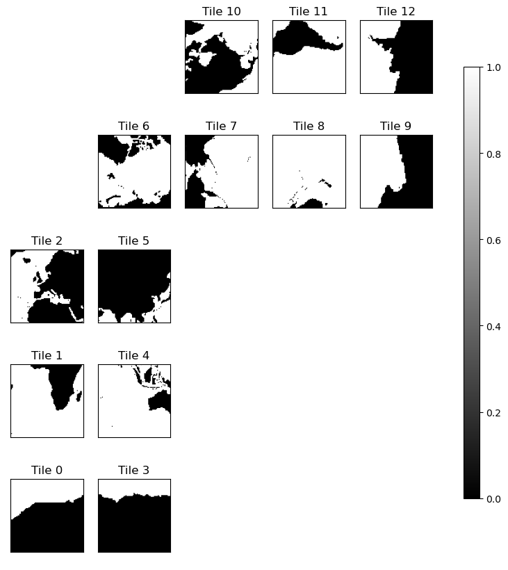
Plot grid parameters using plot_tiles function
Let’s plot two of the model grid parameter fields hFacC (tracer cell thickness factor) and rA (grid cell surface area)
First we plot hFac:
[6]:
ecco.plot_tiles(grid.hFacC.isel(k=0), cmap='gray', show_colorbar=True,);

[7]:
ecco.plot_tiles(grid.rA, cmap='jet', show_colorbar=True);
plt.suptitle('Model grid cell surface area [m^2]')

plt.show()
Plot subset of global domain
Once the file has been “opened” using open_dataset, we can use Dataset.isel to subset the file if we don’t want to plot the full global domain.
[8]:
grid_subset = grid.isel(tile=[1,10,12],k=[0,1,2,3])
grid_subset
[8]:
<xarray.Dataset> Size: 4MB
Dimensions:  (i: 90, i_g: 90, j: 90, j_g: 90, k: 4, k_u: 50, k_l: 50, k_p1: 51,
              tile: 3, nb: 4, nv: 2)
Coordinates: (12/20)
  * i        (i) int32 360B 0 1 2 3 4 5 6 7 8 9 ... 81 82 83 84 85 86 87 88 89
  * i_g      (i_g) int32 360B 0 1 2 3 4 5 6 7 8 9 ... 81 82 83 84 85 86 87 88 89
  * j        (j) int32 360B 0 1 2 3 4 5 6 7 8 9 ... 81 82 83 84 85 86 87 88 89
  * j_g      (j_g) int32 360B 0 1 2 3 4 5 6 7 8 9 ... 81 82 83 84 85 86 87 88 89
  * k        (k) int32 16B 0 1 2 3
  * k_u      (k_u) int32 200B 0 1 2 3 4 5 6 7 8 9 ... 41 42 43 44 45 46 47 48 49
    ...       ...
    Zp1      (k_p1) float32 204B dask.array<chunksize=(51,), meta=np.ndarray>
    Zu       (k_u) float32 200B dask.array<chunksize=(50,), meta=np.ndarray>
    Zl       (k_l) float32 200B dask.array<chunksize=(50,), meta=np.ndarray>
    XC_bnds  (tile, j, i, nb) float32 389kB dask.array<chunksize=(3, 90, 90, 4), meta=np.ndarray>
    YC_bnds  (tile, j, i, nb) float32 389kB dask.array<chunksize=(3, 90, 90, 4), meta=np.ndarray>
    Z_bnds   (k, nv) float32 32B dask.array<chunksize=(4, 2), meta=np.ndarray>
Dimensions without coordinates: nb, nv
Data variables: (12/21)
    CS       (tile, j, i) float32 97kB dask.array<chunksize=(3, 90, 90), meta=np.ndarray>
    SN       (tile, j, i) float32 97kB dask.array<chunksize=(3, 90, 90), meta=np.ndarray>
    rA       (tile, j, i) float32 97kB dask.array<chunksize=(3, 90, 90), meta=np.ndarray>
    dxG      (tile, j_g, i) float32 97kB dask.array<chunksize=(3, 90, 90), meta=np.ndarray>
    dyG      (tile, j, i_g) float32 97kB dask.array<chunksize=(3, 90, 90), meta=np.ndarray>
    Depth    (tile, j, i) float32 97kB dask.array<chunksize=(3, 90, 90), meta=np.ndarray>
    ...       ...
    hFacC    (k, tile, j, i) float32 389kB dask.array<chunksize=(4, 1, 45, 45), meta=np.ndarray>
    hFacW    (k, tile, j, i_g) float32 389kB dask.array<chunksize=(4, 1, 45, 45), meta=np.ndarray>
    hFacS    (k, tile, j_g, i) float32 389kB dask.array<chunksize=(4, 1, 45, 45), meta=np.ndarray>
    maskC    (k, tile, j, i) bool 97kB dask.array<chunksize=(4, 1, 45, 45), meta=np.ndarray>
    maskW    (k, tile, j, i_g) bool 97kB dask.array<chunksize=(4, 1, 45, 45), meta=np.ndarray>
    maskS    (k, tile, j_g, i) bool 97kB dask.array<chunksize=(4, 1, 45, 45), meta=np.ndarray>
Attributes: (12/58)
    acknowledgement:                 This research was carried out by the Jet...
    author:                          Ian Fenty and Ou Wang
    cdm_data_type:                   Grid
    comment:                         Fields provided on the curvilinear lat-l...
    Conventions:                     CF-1.8, ACDD-1.3
    coordinates_comment:             Note: the global 'coordinates' attribute...
    ...                              ...
    references:                      ECCO Consortium, Fukumori, I., Wang, O.,...
    source:                          The ECCO V4r4 state estimate was produce...
    standard_name_vocabulary:        NetCDF Climate and Forecast (CF) Metadat...
    summary:                         This dataset provides geometric paramete...
    title:                           ECCO Geometry Parameters for the Lat-Lon...
uuid: 87ff7d24-86e5-11eb-9c5f-f8f21e2ee3e0- i: 90
- i_g: 90
- j: 90
- j_g: 90
- k: 4
- k_u: 50
- k_l: 50
- k_p1: 51
- tile: 3
- nb: 4
- nv: 2
- i(i)int320 1 2 3 4 5 6 ... 84 85 86 87 88 89
- axis :
- X
- long_name :
- grid index in x for variables at tracer and 'v' locations
- swap_dim :
- XC
- comment :
- In the Arakawa C-grid system, tracer (e.g., THETA) and 'v' variables (e.g., VVEL) have the same x coordinate on the model grid.
- coverage_content_type :
- coordinate
array([ 0, 1, 2, 3, 4, 5, 6, 7, 8, 9, 10, 11, 12, 13, 14, 15, 16, 17, 18, 19, 20, 21, 22, 23, 24, 25, 26, 27, 28, 29, 30, 31, 32, 33, 34, 35, 36, 37, 38, 39, 40, 41, 42, 43, 44, 45, 46, 47, 48, 49, 50, 51, 52, 53, 54, 55, 56, 57, 58, 59, 60, 61, 62, 63, 64, 65, 66, 67, 68, 69, 70, 71, 72, 73, 74, 75, 76, 77, 78, 79, 80, 81, 82, 83, 84, 85, 86, 87, 88, 89], dtype=int32) - i_g(i_g)int320 1 2 3 4 5 6 ... 84 85 86 87 88 89
- axis :
- X
- long_name :
- grid index in x for variables at 'u' and 'g' locations
- c_grid_axis_shift :
- -0.5
- swap_dim :
- XG
- comment :
- In the Arakawa C-grid system, 'u' (e.g., UVEL) and 'g' variables (e.g., XG) have the same x coordinate on the model grid.
- coverage_content_type :
- coordinate
array([ 0, 1, 2, 3, 4, 5, 6, 7, 8, 9, 10, 11, 12, 13, 14, 15, 16, 17, 18, 19, 20, 21, 22, 23, 24, 25, 26, 27, 28, 29, 30, 31, 32, 33, 34, 35, 36, 37, 38, 39, 40, 41, 42, 43, 44, 45, 46, 47, 48, 49, 50, 51, 52, 53, 54, 55, 56, 57, 58, 59, 60, 61, 62, 63, 64, 65, 66, 67, 68, 69, 70, 71, 72, 73, 74, 75, 76, 77, 78, 79, 80, 81, 82, 83, 84, 85, 86, 87, 88, 89], dtype=int32) - j(j)int320 1 2 3 4 5 6 ... 84 85 86 87 88 89
- axis :
- Y
- long_name :
- grid index in y for variables at tracer and 'u' locations
- swap_dim :
- YC
- comment :
- In the Arakawa C-grid system, tracer (e.g., THETA) and 'u' variables (e.g., UVEL) have the same y coordinate on the model grid.
- coverage_content_type :
- coordinate
array([ 0, 1, 2, 3, 4, 5, 6, 7, 8, 9, 10, 11, 12, 13, 14, 15, 16, 17, 18, 19, 20, 21, 22, 23, 24, 25, 26, 27, 28, 29, 30, 31, 32, 33, 34, 35, 36, 37, 38, 39, 40, 41, 42, 43, 44, 45, 46, 47, 48, 49, 50, 51, 52, 53, 54, 55, 56, 57, 58, 59, 60, 61, 62, 63, 64, 65, 66, 67, 68, 69, 70, 71, 72, 73, 74, 75, 76, 77, 78, 79, 80, 81, 82, 83, 84, 85, 86, 87, 88, 89], dtype=int32) - j_g(j_g)int320 1 2 3 4 5 6 ... 84 85 86 87 88 89
- axis :
- Y
- long_name :
- grid index in y for variables at 'v' and 'g' locations
- c_grid_axis_shift :
- -0.5
- swap_dim :
- YG
- comment :
- In the Arakawa C-grid system, 'v' (e.g., VVEL) and 'g' variables (e.g., XG) have the same y coordinate.
- coverage_content_type :
- coordinate
array([ 0, 1, 2, 3, 4, 5, 6, 7, 8, 9, 10, 11, 12, 13, 14, 15, 16, 17, 18, 19, 20, 21, 22, 23, 24, 25, 26, 27, 28, 29, 30, 31, 32, 33, 34, 35, 36, 37, 38, 39, 40, 41, 42, 43, 44, 45, 46, 47, 48, 49, 50, 51, 52, 53, 54, 55, 56, 57, 58, 59, 60, 61, 62, 63, 64, 65, 66, 67, 68, 69, 70, 71, 72, 73, 74, 75, 76, 77, 78, 79, 80, 81, 82, 83, 84, 85, 86, 87, 88, 89], dtype=int32) - k(k)int320 1 2 3
- axis :
- Z
- long_name :
- grid index in z for tracer variables
- swap_dim :
- Z
- coverage_content_type :
- coordinate
array([0, 1, 2, 3], dtype=int32)
- k_u(k_u)int320 1 2 3 4 5 6 ... 44 45 46 47 48 49
- axis :
- Z
- long_name :
- grid index in z corresponding to the bottom face of tracer grid cells ('w' locations)
- c_grid_axis_shift :
- 0.5
- swap_dim :
- Zu
- comment :
- First index corresponds to the bottom face of the uppermost tracer grid cell. The use of 'u' in the variable name follows the MITgcm convention for naming the bottom face of ocean tracer grid cells.
- coverage_content_type :
- coordinate
array([ 0, 1, 2, 3, 4, 5, 6, 7, 8, 9, 10, 11, 12, 13, 14, 15, 16, 17, 18, 19, 20, 21, 22, 23, 24, 25, 26, 27, 28, 29, 30, 31, 32, 33, 34, 35, 36, 37, 38, 39, 40, 41, 42, 43, 44, 45, 46, 47, 48, 49], dtype=int32) - k_l(k_l)int320 1 2 3 4 5 6 ... 44 45 46 47 48 49
- axis :
- Z
- long_name :
- grid index in z corresponding to the top face of tracer grid cells ('w' locations)
- c_grid_axis_shift :
- -0.5
- swap_dim :
- Zl
- comment :
- First index corresponds to the top face of the uppermost tracer grid cell. The use of 'l' in the variable name follows the MITgcm convention for naming the top face of ocean tracer grid cells.
- coverage_content_type :
- coordinate
array([ 0, 1, 2, 3, 4, 5, 6, 7, 8, 9, 10, 11, 12, 13, 14, 15, 16, 17, 18, 19, 20, 21, 22, 23, 24, 25, 26, 27, 28, 29, 30, 31, 32, 33, 34, 35, 36, 37, 38, 39, 40, 41, 42, 43, 44, 45, 46, 47, 48, 49], dtype=int32) - k_p1(k_p1)int320 1 2 3 4 5 6 ... 45 46 47 48 49 50
- axis :
- Z
- long_name :
- grid index in z for variables at 'w' locations
- c_grid_axis_shift :
- [-0.5 0.5]
- swap_dim :
- Zp1
- comment :
- Includes top of uppermost model tracer cell (k_p1=0) and bottom of lowermost tracer cell (k_p1=51).
- coverage_content_type :
- coordinate
array([ 0, 1, 2, 3, 4, 5, 6, 7, 8, 9, 10, 11, 12, 13, 14, 15, 16, 17, 18, 19, 20, 21, 22, 23, 24, 25, 26, 27, 28, 29, 30, 31, 32, 33, 34, 35, 36, 37, 38, 39, 40, 41, 42, 43, 44, 45, 46, 47, 48, 49, 50], dtype=int32) - tile(tile)int321 10 12
- long_name :
- lat-lon-cap tile index
- comment :
- The ECCO V4 horizontal model grid is divided into 13 tiles of 90x90 cells for convenience.
- coverage_content_type :
- coordinate
array([ 1, 10, 12], dtype=int32)
- XC(tile, j, i)float32dask.array<chunksize=(3, 90, 90), meta=np.ndarray>
- long_name :
- longitude of tracer grid cell center
- units :
- degrees_east
- coordinate :
- YC XC
- bounds :
- XC_bnds
- comment :
- nonuniform grid spacing
- coverage_content_type :
- coordinate
- standard_name :
- longitude
Array Chunk Bytes 94.92 kiB 94.92 kiB Shape (3, 90, 90) (3, 90, 90) Dask graph 1 chunks in 3 graph layers Data type float32 numpy.ndarray - YC(tile, j, i)float32dask.array<chunksize=(3, 90, 90), meta=np.ndarray>
- long_name :
- latitude of tracer grid cell center
- units :
- degrees_north
- coordinate :
- YC XC
- bounds :
- YC_bnds
- comment :
- nonuniform grid spacing
- coverage_content_type :
- coordinate
- standard_name :
- latitude
Array Chunk Bytes 94.92 kiB 94.92 kiB Shape (3, 90, 90) (3, 90, 90) Dask graph 1 chunks in 3 graph layers Data type float32 numpy.ndarray - XG(tile, j_g, i_g)float32dask.array<chunksize=(3, 90, 90), meta=np.ndarray>
- long_name :
- longitude of 'southwest' corner of tracer grid cell
- units :
- degrees_east
- coordinate :
- YG XG
- comment :
- Nonuniform grid spacing. Note: 'southwest' does not correspond to geographic orientation but is used for convenience to describe the computational grid. See MITgcm dcoumentation for details.
- coverage_content_type :
- coordinate
- standard_name :
- longitude
Array Chunk Bytes 94.92 kiB 94.92 kiB Shape (3, 90, 90) (3, 90, 90) Dask graph 1 chunks in 3 graph layers Data type float32 numpy.ndarray - YG(tile, j_g, i_g)float32dask.array<chunksize=(3, 90, 90), meta=np.ndarray>
- long_name :
- latitude of 'southwest' corner of tracer grid cell
- units :
- degrees_north
- comment :
- Nonuniform grid spacing. Note: 'southwest' does not correspond to geographic orientation but is used for convenience to describe the computational grid. See MITgcm dcoumentation for details.
- coverage_content_type :
- coordinate
- standard_name :
- latitude
Array Chunk Bytes 94.92 kiB 94.92 kiB Shape (3, 90, 90) (3, 90, 90) Dask graph 1 chunks in 3 graph layers Data type float32 numpy.ndarray - Z(k)float32dask.array<chunksize=(4,), meta=np.ndarray>
- long_name :
- depth of tracer grid cell center
- units :
- m
- positive :
- up
- bounds :
- Z_bnds
- comment :
- Non-uniform vertical spacing.
- coverage_content_type :
- coordinate
- standard_name :
- depth
Array Chunk Bytes 16 B 16 B Shape (4,) (4,) Dask graph 1 chunks in 3 graph layers Data type float32 numpy.ndarray - Zp1(k_p1)float32dask.array<chunksize=(51,), meta=np.ndarray>
- long_name :
- depth of top/bottom face of tracer grid cell
- units :
- m
- positive :
- up
- comment :
- Contains one element more than the number of vertical layers. First element is 0m, the depth of the top face of the uppermost grid cell. Last element is the depth of the bottom face of the deepest grid cell.
- coverage_content_type :
- coordinate
- standard_name :
- depth
Array Chunk Bytes 204 B 204 B Shape (51,) (51,) Dask graph 1 chunks in 2 graph layers Data type float32 numpy.ndarray - Zu(k_u)float32dask.array<chunksize=(50,), meta=np.ndarray>
- long_name :
- depth of bottom face of tracer grid cell
- units :
- m
- positive :
- up
- comment :
- First element is -10m, the depth of the bottom face of the uppermost tracer grid cell. Last element is the depth of the bottom face of the deepest grid cell. The use of 'u' in the variable name follows the MITgcm convention for naming the bottom face of ocean tracer grid cells.
- coverage_content_type :
- coordinate
- standard_name :
- depth
Array Chunk Bytes 200 B 200 B Shape (50,) (50,) Dask graph 1 chunks in 2 graph layers Data type float32 numpy.ndarray - Zl(k_l)float32dask.array<chunksize=(50,), meta=np.ndarray>
- long_name :
- depth of top face of tracer grid cell
- units :
- m
- positive :
- up
- comment :
- First element is 0m, the depth of the top face of the uppermost tracer grid cell (i.e., the ocean surface). Last element is the depth of the top face of the deepest grid cell. The use of 'l' in the variable name follows the MITgcm convention for naming the top face of ocean tracer grid cells.
- coverage_content_type :
- coordinate
- standard_name :
- depth
Array Chunk Bytes 200 B 200 B Shape (50,) (50,) Dask graph 1 chunks in 2 graph layers Data type float32 numpy.ndarray - XC_bnds(tile, j, i, nb)float32dask.array<chunksize=(3, 90, 90, 4), meta=np.ndarray>
- comment :
- Bounds array follows CF conventions. XC_bnds[i,j,0] = 'southwest' corner (j-1, i-1), XC_bnds[i,j,1] = 'southeast' corner (j-1, i+1), XC_bnds[i,j,2] = 'northeast' corner (j+1, i+1), XC_bnds[i,j,3] = 'northwest' corner (j+1, i-1). Note: 'southwest', 'southeast', northwest', and 'northeast' do not correspond to geographic orientation but are used for convenience to describe the computational grid. See MITgcm dcoumentation for details.
- coverage_content_type :
- coordinate
- long_name :
- longitudes of tracer grid cell corners
Array Chunk Bytes 379.69 kiB 379.69 kiB Shape (3, 90, 90, 4) (3, 90, 90, 4) Dask graph 1 chunks in 3 graph layers Data type float32 numpy.ndarray - YC_bnds(tile, j, i, nb)float32dask.array<chunksize=(3, 90, 90, 4), meta=np.ndarray>
- comment :
- Bounds array follows CF conventions. YC_bnds[i,j,0] = 'southwest' corner (j-1, i-1), YC_bnds[i,j,1] = 'southeast' corner (j-1, i+1), YC_bnds[i,j,2] = 'northeast' corner (j+1, i+1), YC_bnds[i,j,3] = 'northwest' corner (j+1, i-1). Note: 'southwest', 'southeast', northwest', and 'northeast' do not correspond to geographic orientation but are used for convenience to describe the computational grid. See MITgcm dcoumentation for details.
- coverage_content_type :
- coordinate
- long_name :
- latitudes of tracer grid cell corners
Array Chunk Bytes 379.69 kiB 379.69 kiB Shape (3, 90, 90, 4) (3, 90, 90, 4) Dask graph 1 chunks in 3 graph layers Data type float32 numpy.ndarray - Z_bnds(k, nv)float32dask.array<chunksize=(4, 2), meta=np.ndarray>
- comment :
- One pair of depths for each vertical level.
- coverage_content_type :
- coordinate
- long_name :
- depths of top and bottom faces of tracer grid cell
Array Chunk Bytes 32 B 32 B Shape (4, 2) (4, 2) Dask graph 1 chunks in 3 graph layers Data type float32 numpy.ndarray
- CS(tile, j, i)float32dask.array<chunksize=(3, 90, 90), meta=np.ndarray>
- long_name :
- cosine of tracer grid cell orientation vs geographical north
- units :
- 1
- coordinate :
- YC XC
- coverage_content_type :
- modelResult
- comment :
- CS and SN are required to calculate the geographic (meridional, zonal) components of vectors on the curvilinear model grid. Note: for vector R with components R_x and R_y: R_{east} = CS R_x - SN R_y. R_{north} = SN R_x + CS R_y
Array Chunk Bytes 94.92 kiB 94.92 kiB Shape (3, 90, 90) (3, 90, 90) Dask graph 1 chunks in 3 graph layers Data type float32 numpy.ndarray - SN(tile, j, i)float32dask.array<chunksize=(3, 90, 90), meta=np.ndarray>
- long_name :
- sine of tracer grid cell orientation vs geographical north
- units :
- 1
- coordinate :
- YC XC
- coverage_content_type :
- modelResult
- comment :
- CS and SN are required to calculate the geographic (meridional, zonal) components of vectors on the curvilinear model grid. Note: for vector R with components R_x and R_y in local grid directions x and y, the geographical eastward component R_{east} = CS R_x - SN R_y. The geographical northward component R_{north} = SN R_x + CS R_y.
Array Chunk Bytes 94.92 kiB 94.92 kiB Shape (3, 90, 90) (3, 90, 90) Dask graph 1 chunks in 3 graph layers Data type float32 numpy.ndarray - rA(tile, j, i)float32dask.array<chunksize=(3, 90, 90), meta=np.ndarray>
- long_name :
- area of tracer grid cell
- units :
- m2
- coordinate :
- YC XC
- coverage_content_type :
- modelResult
- standard_name :
- cell_area
Array Chunk Bytes 94.92 kiB 94.92 kiB Shape (3, 90, 90) (3, 90, 90) Dask graph 1 chunks in 3 graph layers Data type float32 numpy.ndarray - dxG(tile, j_g, i)float32dask.array<chunksize=(3, 90, 90), meta=np.ndarray>
- long_name :
- distance between 'southwest' and 'southeast' corners of the tracer grid cell
- units :
- m
- coordinate :
- YG XC
- coverage_content_type :
- modelResult
- comment :
- Alternatively, the length of 'south' side of tracer grid cell. Note: 'south', 'southwest', and 'southeast' do not correspond to geographic orientation but are used for convenience to describe the computational grid. See MITgcm documentation for details.
Array Chunk Bytes 94.92 kiB 94.92 kiB Shape (3, 90, 90) (3, 90, 90) Dask graph 1 chunks in 3 graph layers Data type float32 numpy.ndarray - dyG(tile, j, i_g)float32dask.array<chunksize=(3, 90, 90), meta=np.ndarray>
- long_name :
- distance between 'southwest' and 'northwest' corners of the tracer grid cell
- units :
- m
- coordinate :
- YC XG
- coverage_content_type :
- modelResult
- comment :
- Alternatively, the length of 'west' side of tracer grid cell. Note: 'west, 'southwest', and 'northwest' do not correspond to geographic orientation but are used for convenience to describe the computational grid. See MITgcm documentation for details.
Array Chunk Bytes 94.92 kiB 94.92 kiB Shape (3, 90, 90) (3, 90, 90) Dask graph 1 chunks in 3 graph layers Data type float32 numpy.ndarray - Depth(tile, j, i)float32dask.array<chunksize=(3, 90, 90), meta=np.ndarray>
- long_name :
- model seafloor depth below ocean surface at rest
- units :
- m
- coordinate :
- XC YC
- coverage_content_type :
- modelResult
- standard_name :
- sea_floor_depth_below_geoid
- comment :
- Model sea surface height (SSH) of 0m corresponds to an ocean surface at rest relative to the geoid. Depth corresponds to seafloor depth below geoid. Note: the MITgcm used by ECCO V4r4 implements 'partial cells' so the actual model seafloor depth may differ from the seafloor depth provided by the input bathymetry file.
Array Chunk Bytes 94.92 kiB 94.92 kiB Shape (3, 90, 90) (3, 90, 90) Dask graph 1 chunks in 3 graph layers Data type float32 numpy.ndarray - rAz(tile, j_g, i_g)float32dask.array<chunksize=(3, 90, 90), meta=np.ndarray>
- long_name :
- area of vorticity 'g' grid cell
- units :
- m2
- coordinate :
- YG XG
- coverage_content_type :
- modelResult
- standard_name :
- cell_area
- comment :
- Vorticity cells are staggered in space relative to tracer cells, nominally situated on tracer cell corners. Vorticity cell (i,j) is located at the 'southwest' corner of tracer grid cell (i, j). Note: 'southwest' does not correspond to geographic orientation but is used for convenience to describe the computational grid. See MITgcm documentation for details.
Array Chunk Bytes 94.92 kiB 94.92 kiB Shape (3, 90, 90) (3, 90, 90) Dask graph 1 chunks in 3 graph layers Data type float32 numpy.ndarray - dxC(tile, j, i_g)float32dask.array<chunksize=(3, 90, 90), meta=np.ndarray>
- long_name :
- distance between centers of adjacent tracer grid cells in the 'x' direction
- units :
- m
- coordinate :
- YC XG
- coverage_content_type :
- modelResult
- comment :
- Alternatively, the length of 'north' side of vorticity grid cells. Note: 'north' does not correspond to geographic orientation but is used for convenience to describe the computational grid. See MITgcm documentation for details.
Array Chunk Bytes 94.92 kiB 94.92 kiB Shape (3, 90, 90) (3, 90, 90) Dask graph 1 chunks in 3 graph layers Data type float32 numpy.ndarray - dyC(tile, j_g, i)float32dask.array<chunksize=(3, 90, 90), meta=np.ndarray>
- long_name :
- distance between centers of adjacent tracer grid cells in the 'y' direction
- units :
- m
- coordinate :
- YG XC
- coverage_content_type :
- modelResult
- comment :
- Alternatively, the length of 'east' side of vorticity grid cells. Note: 'east' does not correspond to geographic orientation but is used for convenience to describe the computational grid. See MITgcm documentation for details.
Array Chunk Bytes 94.92 kiB 94.92 kiB Shape (3, 90, 90) (3, 90, 90) Dask graph 1 chunks in 3 graph layers Data type float32 numpy.ndarray - rAw(tile, j, i_g)float32dask.array<chunksize=(3, 90, 90), meta=np.ndarray>
- long_name :
- area of 'v' grid cell
- units :
- m2
- coordinate :
- YG XC
- coverage_content_type :
- modelResult
- standard_name :
- cell_area
- comment :
- Model 'v' grid cells are staggered in space between adjacent tracer grid cells in the 'x' direction. 'v' grid cell (i,j) is situated at the 'west' edge of tracer grid cell (i, j). Note: 'west' does not correspond to geographic orientation but is used for convenience to describe the computational grid. See MITgcm documentation for details.
Array Chunk Bytes 94.92 kiB 94.92 kiB Shape (3, 90, 90) (3, 90, 90) Dask graph 1 chunks in 3 graph layers Data type float32 numpy.ndarray - rAs(tile, j_g, i)float32dask.array<chunksize=(3, 90, 90), meta=np.ndarray>
- long_name :
- area of 'u' grid cell
- units :
- m2
- coverage_content_type :
- modelResult
- standard_name :
- cell_area
- comment :
- Model 'u' grid cells are staggered in space between adjacent tracer grid cells in the 'y' direction. 'u' grid cell (i,j) is situated at the 'south' edge of tracer grid cell (i, j). Note: 'south' does not correspond to geographic orientation but is used for convenience to describe the computational grid. See MITgcm documentation for details.
Array Chunk Bytes 94.92 kiB 94.92 kiB Shape (3, 90, 90) (3, 90, 90) Dask graph 1 chunks in 3 graph layers Data type float32 numpy.ndarray - drC(k_p1)float32dask.array<chunksize=(51,), meta=np.ndarray>
- long_name :
- distance between the centers of adjacent tracer grid cells in the 'z' direction
- units :
- m
- coverage_content_type :
- modelResult
- comment :
- The first element corresponds to the distance between the depth of the center of the uppermost model grid cell and the surface.
Array Chunk Bytes 204 B 204 B Shape (51,) (51,) Dask graph 1 chunks in 2 graph layers Data type float32 numpy.ndarray - drF(k)float32dask.array<chunksize=(4,), meta=np.ndarray>
- long_name :
- distance between the upper and lower interfaces of the model grid cell
- units :
- m
- coverage_content_type :
- modelResult
- standard_name :
- cell_thickness
- comment :
- Nominal grid cell thickness. Note: in the z* coordinate system used in ECCO V4, actual tracer grid cell thickness, h, varies through time as h(i,j,k,t)= drF(k) hfacC(i,j,k,t).
Array Chunk Bytes 16 B 16 B Shape (4,) (4,) Dask graph 1 chunks in 3 graph layers Data type float32 numpy.ndarray - PHrefC(k)float32dask.array<chunksize=(4,), meta=np.ndarray>
- long_name :
- reference ocean hydrostatic pressure at tracer grid cell center
- units :
- m2 s-2
- coverage_content_type :
- modelResult
- comment :
- PHrefC = p_ref (k) / rhoConst = rhoConst g z(k) / rhoConst = g z(k), where p_ref(k) is reference hydrostatic ocean pressure at center of tracer grid cell k, rhoConst is reference density (1029 kg m-3), g is acceleration due to gravity (9.81 m s-2), and z(k) is depth at center of tracer grid cell k. Units: p:[kg m-1 s-2], rhoConst:[kg m-3], g:[m s-2], z_m(t):[m]. Note: does not include atmospheric pressure loading. Quantity referred to in some contexts as hydrostatic pressure potential. PHIHYDcR is anomaly of PHrefC.
Array Chunk Bytes 16 B 16 B Shape (4,) (4,) Dask graph 1 chunks in 3 graph layers Data type float32 numpy.ndarray - PHrefF(k_p1)float32dask.array<chunksize=(51,), meta=np.ndarray>
- long_name :
- reference ocean hydrostatic pressure at tracer grid cell top/bottom interface
- units :
- m2 s-2
- coverage_content_type :
- modelResult
- comment :
- PHrefF = p_ref (k_l) / rhoConst = rhoConst g z(k_l) / rhoConst = g z(k_l), where p_ref(k_l) is reference hydrostatic ocean pressure at lower interface of tracer grid cell k, rhoConst is reference density (1029 kg m-3), g is acceleration due to gravity (9.81 m s-2), and z(k) is depth at center of tracer grid cell k. Units: p:[kg m-1 s-2], rhoConst:[kg m-3], g:[m s-2], z_m(t):[m]. Note: does not include atmospheric pressure loading. Quantity referred to in some contexts as hydrostatic pressure potential. See PHrefC
Array Chunk Bytes 204 B 204 B Shape (51,) (51,) Dask graph 1 chunks in 2 graph layers Data type float32 numpy.ndarray - hFacC(k, tile, j, i)float32dask.array<chunksize=(4, 1, 45, 45), meta=np.ndarray>
- long_name :
- vertical open fraction of tracer grid cell
- coverage_content_type :
- modelResult
- units :
- 1
- comment :
- Tracer grid cells may be fractionally closed in the vertical. The open vertical fraction is hFacC. The model allows for partially-filled cells to represent topographic variations more smoothly (hFacC < 1). Completely closed (dry) tracer grid cells have hFacC = 0. Note: the model z* coordinate system allows hFacC to vary through time. A time-invariant hFacC field is provided for reference.
Array Chunk Bytes 379.69 kiB 63.28 kiB Shape (4, 3, 90, 90) (4, 2, 45, 45) Dask graph 8 chunks in 4 graph layers Data type float32 numpy.ndarray - hFacW(k, tile, j, i_g)float32dask.array<chunksize=(4, 1, 45, 45), meta=np.ndarray>
- long_name :
- vertical open fraction of tracer grid cell 'west' face
- coverage_content_type :
- modelResult
- units :
- 1
- comment :
- The 'west' face of tracer grid cells may be fractionally closed in the vertical. The open vertical fraction is hFacW. The model allows for partially-filled cells for smoother representation of seafloor topography. Tracer grid cells adjacent in the 'x' direction that are partially closed in the vertical have hFacW < 1. The model z* coordinate system used by the model permits hFacC, and therefore hFacW, to vary through time. A time-invariant hFacW field is provided for reference. Note: The term 'west' does not correspond to geographic orientation but is used for convenience to describe the computational grid. See MITgcm documentation for details.
Array Chunk Bytes 379.69 kiB 63.28 kiB Shape (4, 3, 90, 90) (4, 2, 45, 45) Dask graph 8 chunks in 4 graph layers Data type float32 numpy.ndarray - hFacS(k, tile, j_g, i)float32dask.array<chunksize=(4, 1, 45, 45), meta=np.ndarray>
- long_name :
- vertical open fraction of tracer grid cell 'south' face
- coverage_content_type :
- modelResult
- units :
- 1
- comment :
- The 'south' face of tracer grid cells may be fractionally closed in the vertical. The open vertical fraction is hFacS. The model allows for partially-filled cells for smoother representation of seafloor topography. Tracer grid cells adjacent in the 'y' direction that are partially closed in the vertical have hFacS < 1. The model z* coordinate system used by the model permits hFacC, and therefore hFacS, to vary through time. A time-invariant hFacS field is provided for reference. Note: The term 'south' does not correspond to geographic orientation but is used for convenience to describe the computational grid. See MITgcm documentation for details.
Array Chunk Bytes 379.69 kiB 63.28 kiB Shape (4, 3, 90, 90) (4, 2, 45, 45) Dask graph 8 chunks in 4 graph layers Data type float32 numpy.ndarray - maskC(k, tile, j, i)booldask.array<chunksize=(4, 1, 45, 45), meta=np.ndarray>
- long_name :
- wet/dry boolean mask for tracer grid cell
- coverage_content_type :
- modelResult
- comment :
- True for tracer grid cells with nonzero open vertical fraction (hFacC > 0), otherwise False. Although hFacC can vary though time, cells will never close if starting open and will never open if starting closed: hFacC(i,j,k,t) > 0 for all t, if hFacC(i,j,k,t=0) and hFacC(i,j,k,t) = 0 for all t, if hFacC(i,j,k,t=0) = 0. Therefore, maskC is time invariant.
Array Chunk Bytes 94.92 kiB 15.82 kiB Shape (4, 3, 90, 90) (4, 2, 45, 45) Dask graph 8 chunks in 4 graph layers Data type bool numpy.ndarray - maskW(k, tile, j, i_g)booldask.array<chunksize=(4, 1, 45, 45), meta=np.ndarray>
- long_name :
- wet/dry boolean mask for 'west' face of tracer grid cell
- coverage_content_type :
- modelResult
- comment :
- True for grid cells with nonzero open vertical fraction along their 'west' face (hFacW > 0), otherwise False. Although hFacW can vary though time, cells will never close if starting open and will never open if starting closed: hFacW(i,j,k,t) > 0 for all t, if hFacW(i,j,k,t=0) and hFacW(i,j,k,t) = 0 for all t, if hFacW(i,j,k,t=0) = 0. Therefore, maskW is time invariant. Note:
Array Chunk Bytes 94.92 kiB 15.82 kiB Shape (4, 3, 90, 90) (4, 2, 45, 45) Dask graph 8 chunks in 4 graph layers Data type bool numpy.ndarray - maskS(k, tile, j_g, i)booldask.array<chunksize=(4, 1, 45, 45), meta=np.ndarray>
- long_name :
- wet/dry boolean mask for 'south' face of tracer grid cell
- coverage_content_type :
- modelResult
- comment :
- True for grid cells with nonzero open vertical fraction along their 'south' face (hFacS > 0), otherwise False. Although hFacS can vary though time, cells will never close if starting open and will never open if starting closed: hFacS(i,j,k,t) > 0 for all t, if hFacS(i,j,k,t=0) and hFacS(i,j,k,t) = 0 for all t, if hFacS(i,j,k,t=0) = 0. Therefore, maskS is time invariant. Note:
Array Chunk Bytes 94.92 kiB 15.82 kiB Shape (4, 3, 90, 90) (4, 2, 45, 45) Dask graph 8 chunks in 4 graph layers Data type bool numpy.ndarray
- iPandasIndex
PandasIndex(Index([ 0, 1, 2, 3, 4, 5, 6, 7, 8, 9, 10, 11, 12, 13, 14, 15, 16, 17, 18, 19, 20, 21, 22, 23, 24, 25, 26, 27, 28, 29, 30, 31, 32, 33, 34, 35, 36, 37, 38, 39, 40, 41, 42, 43, 44, 45, 46, 47, 48, 49, 50, 51, 52, 53, 54, 55, 56, 57, 58, 59, 60, 61, 62, 63, 64, 65, 66, 67, 68, 69, 70, 71, 72, 73, 74, 75, 76, 77, 78, 79, 80, 81, 82, 83, 84, 85, 86, 87, 88, 89], dtype='int32', name='i')) - i_gPandasIndex
PandasIndex(Index([ 0, 1, 2, 3, 4, 5, 6, 7, 8, 9, 10, 11, 12, 13, 14, 15, 16, 17, 18, 19, 20, 21, 22, 23, 24, 25, 26, 27, 28, 29, 30, 31, 32, 33, 34, 35, 36, 37, 38, 39, 40, 41, 42, 43, 44, 45, 46, 47, 48, 49, 50, 51, 52, 53, 54, 55, 56, 57, 58, 59, 60, 61, 62, 63, 64, 65, 66, 67, 68, 69, 70, 71, 72, 73, 74, 75, 76, 77, 78, 79, 80, 81, 82, 83, 84, 85, 86, 87, 88, 89], dtype='int32', name='i_g')) - jPandasIndex
PandasIndex(Index([ 0, 1, 2, 3, 4, 5, 6, 7, 8, 9, 10, 11, 12, 13, 14, 15, 16, 17, 18, 19, 20, 21, 22, 23, 24, 25, 26, 27, 28, 29, 30, 31, 32, 33, 34, 35, 36, 37, 38, 39, 40, 41, 42, 43, 44, 45, 46, 47, 48, 49, 50, 51, 52, 53, 54, 55, 56, 57, 58, 59, 60, 61, 62, 63, 64, 65, 66, 67, 68, 69, 70, 71, 72, 73, 74, 75, 76, 77, 78, 79, 80, 81, 82, 83, 84, 85, 86, 87, 88, 89], dtype='int32', name='j')) - j_gPandasIndex
PandasIndex(Index([ 0, 1, 2, 3, 4, 5, 6, 7, 8, 9, 10, 11, 12, 13, 14, 15, 16, 17, 18, 19, 20, 21, 22, 23, 24, 25, 26, 27, 28, 29, 30, 31, 32, 33, 34, 35, 36, 37, 38, 39, 40, 41, 42, 43, 44, 45, 46, 47, 48, 49, 50, 51, 52, 53, 54, 55, 56, 57, 58, 59, 60, 61, 62, 63, 64, 65, 66, 67, 68, 69, 70, 71, 72, 73, 74, 75, 76, 77, 78, 79, 80, 81, 82, 83, 84, 85, 86, 87, 88, 89], dtype='int32', name='j_g')) - kPandasIndex
PandasIndex(Index([0, 1, 2, 3], dtype='int32', name='k'))
- k_uPandasIndex
PandasIndex(Index([ 0, 1, 2, 3, 4, 5, 6, 7, 8, 9, 10, 11, 12, 13, 14, 15, 16, 17, 18, 19, 20, 21, 22, 23, 24, 25, 26, 27, 28, 29, 30, 31, 32, 33, 34, 35, 36, 37, 38, 39, 40, 41, 42, 43, 44, 45, 46, 47, 48, 49], dtype='int32', name='k_u')) - k_lPandasIndex
PandasIndex(Index([ 0, 1, 2, 3, 4, 5, 6, 7, 8, 9, 10, 11, 12, 13, 14, 15, 16, 17, 18, 19, 20, 21, 22, 23, 24, 25, 26, 27, 28, 29, 30, 31, 32, 33, 34, 35, 36, 37, 38, 39, 40, 41, 42, 43, 44, 45, 46, 47, 48, 49], dtype='int32', name='k_l')) - k_p1PandasIndex
PandasIndex(Index([ 0, 1, 2, 3, 4, 5, 6, 7, 8, 9, 10, 11, 12, 13, 14, 15, 16, 17, 18, 19, 20, 21, 22, 23, 24, 25, 26, 27, 28, 29, 30, 31, 32, 33, 34, 35, 36, 37, 38, 39, 40, 41, 42, 43, 44, 45, 46, 47, 48, 49, 50], dtype='int32', name='k_p1')) - tilePandasIndex
PandasIndex(Index([1, 10, 12], dtype='int32', name='tile'))
- acknowledgement :
- This research was carried out by the Jet Propulsion Laboratory, managed by the California Institute of Technology under a contract with the National Aeronautics and Space Administration.
- author :
- Ian Fenty and Ou Wang
- cdm_data_type :
- Grid
- comment :
- Fields provided on the curvilinear lat-lon-cap 90 (llc90) native grid used in the ECCO model.
- Conventions :
- CF-1.8, ACDD-1.3
- coordinates_comment :
- Note: the global 'coordinates' attribute describes auxillary coordinates.
- creator_email :
- ecco-group@mit.edu
- creator_institution :
- NASA Jet Propulsion Laboratory (JPL)
- creator_name :
- ECCO Consortium
- creator_type :
- group
- creator_url :
- https://ecco-group.org
- date_created :
- 2021-03-16T22:56:35
- date_issued :
- 2021-03-16T22:56:35
- date_metadata_modified :
- 2021-03-16T22:56:35
- date_modified :
- 2021-03-16T22:56:35
- geospatial_bounds_crs :
- EPSG:4326
- geospatial_lat_max :
- 90.0
- geospatial_lat_min :
- -90.0
- geospatial_lat_resolution :
- variable
- geospatial_lat_units :
- degrees_north
- geospatial_lon_max :
- 180.0
- geospatial_lon_min :
- -180.0
- geospatial_lon_resolution :
- variable
- geospatial_lon_units :
- degrees_east
- geospatial_vertical_max :
- 0.0
- geospatial_vertical_min :
- -6134.5
- geospatial_vertical_positive :
- up
- geospatial_vertical_resolution :
- variable
- geospatial_vertical_units :
- meter
- history :
- Inaugural release of an ECCO Central Estimate solution to PO.DAAC
- id :
- 10.5067/ECL5A-GRD44
- institution :
- NASA Jet Propulsion Laboratory (JPL)
- instrument_vocabulary :
- GCMD instrument keywords
- keywords :
- EARTH SCIENCE SERVICES > MODELS > EARTH SCIENCE REANALYSES/ASSIMILATION MODELS
- keywords_vocabulary :
- NASA Global Change Master Directory (GCMD) Science Keywords
- license :
- Public Domain
- metadata_link :
- https://cmr.earthdata.nasa.gov/search/collections.umm_json?ShortName=ECCO_L4_GEOMETRY_LLC0090GRID_V4R4
- naming_authority :
- gov.nasa.jpl
- platform :
- ERS-1/2, TOPEX/Poseidon, Geosat Follow-On (GFO), ENVISAT, Jason-1, Jason-2, CryoSat-2, SARAL/AltiKa, Jason-3, AVHRR, Aquarius, SSM/I, SSMIS, GRACE, DTU17MDT, Argo, WOCE, GO-SHIP, MEOP, Ice Tethered Profilers (ITP)
- platform_vocabulary :
- GCMD platform keywords
- processing_level :
- L4
- product_name :
- GRID_GEOMETRY_ECCO_V4r4_native_llc0090.nc
- product_time_coverage_end :
- 2018-01-01T00:00:00
- product_time_coverage_start :
- 1992-01-01T12:00:00
- product_version :
- Version 4, Release 4
- program :
- NASA Physical Oceanography, Cryosphere, Modeling, Analysis, and Prediction (MAP)
- project :
- Estimating the Circulation and Climate of the Ocean (ECCO)
- publisher_email :
- podaac@podaac.jpl.nasa.gov
- publisher_institution :
- PO.DAAC
- publisher_name :
- Physical Oceanography Distributed Active Archive Center (PO.DAAC)
- publisher_type :
- institution
- publisher_url :
- https://podaac.jpl.nasa.gov
- references :
- ECCO Consortium, Fukumori, I., Wang, O., Fenty, I., Forget, G., Heimbach, P., & Ponte, R. M. 2020. Synopsis of the ECCO Central Production Global Ocean and Sea-Ice State Estimate (Version 4 Release 4). doi:10.5281/zenodo.3765928
- source :
- The ECCO V4r4 state estimate was produced by fitting a free-running solution of the MITgcm (checkpoint 66g) to satellite and in situ observational data in a least squares sense using the adjoint method
- standard_name_vocabulary :
- NetCDF Climate and Forecast (CF) Metadata Convention
- summary :
- This dataset provides geometric parameters for the lat-lon-cap 90 (llc90) native model grid from the ECCO Version 4 Release 4 (V4r4) ocean and sea-ice state estimate. Parameters include areas and lengths of grid cell sides, horizontal and vertical coordinates of grid cell centers and corners, grid rotation angles, and global domain geometry including bathymetry and land/ocean masks. Estimating the Circulation and Climate of the Ocean (ECCO) state estimates are dynamically and kinematically-consistent reconstructions of the three-dimensional, time-evolving ocean, sea-ice, and surface atmospheric states. ECCO V4r4 is a free-running solution of a global, nominally 1-degree configuration of the MIT general circulation model (MITgcm) that has been fit to observations in a least-squares sense. Observational data constraints used in V4r4 include sea surface height (SSH) from satellite altimeters [ERS-1/2, TOPEX/Poseidon, GFO, ENVISAT, Jason-1,2,3, CryoSat-2, and SARAL/AltiKa]; sea surface temperature (SST) from satellite radiometers [AVHRR], sea surface salinity (SSS) from the Aquarius satellite radiometer/scatterometer, ocean bottom pressure (OBP) from the GRACE satellite gravimeter; sea-ice concentration from satellite radiometers [SSM/I and SSMIS], and in-situ ocean temperature and salinity measured with conductivity-temperature-depth (CTD) sensors and expendable bathythermographs (XBTs) from several programs [e.g., WOCE, GO-SHIP, Argo, and others] and platforms [e.g., research vessels, gliders, moorings, ice-tethered profilers, and instrumented pinnipeds]. V4r4 covers the period 1992-01-01T12:00:00 to 2018-01-01T00:00:00.
- title :
- ECCO Geometry Parameters for the Lat-Lon-Cap 90 (llc90) Native Model Grid (Version 4 Release 4)
- uuid :
- 87ff7d24-86e5-11eb-9c5f-f8f21e2ee3e0
Notice that grid_subset only has 3 tiles (1, 10, 12) and 4 depth levels (0, 1, 2, 3), as expected. The subset indices can also be passed to isel as a Python dictionary, with the same result.
[9]:
subset_ind = {'tile':[1,10,12],'k':[0,1,2,3]}

grid_subset = grid.isel(subset_ind)
grid_subset
[9]:
<xarray.Dataset> Size: 4MB
Dimensions:  (i: 90, i_g: 90, j: 90, j_g: 90, k: 4, k_u: 50, k_l: 50, k_p1: 51,
              tile: 3, nb: 4, nv: 2)
Coordinates: (12/20)
  * i        (i) int32 360B 0 1 2 3 4 5 6 7 8 9 ... 81 82 83 84 85 86 87 88 89
  * i_g      (i_g) int32 360B 0 1 2 3 4 5 6 7 8 9 ... 81 82 83 84 85 86 87 88 89
  * j        (j) int32 360B 0 1 2 3 4 5 6 7 8 9 ... 81 82 83 84 85 86 87 88 89
  * j_g      (j_g) int32 360B 0 1 2 3 4 5 6 7 8 9 ... 81 82 83 84 85 86 87 88 89
  * k        (k) int32 16B 0 1 2 3
  * k_u      (k_u) int32 200B 0 1 2 3 4 5 6 7 8 9 ... 41 42 43 44 45 46 47 48 49
    ...       ...
    Zp1      (k_p1) float32 204B dask.array<chunksize=(51,), meta=np.ndarray>
    Zu       (k_u) float32 200B dask.array<chunksize=(50,), meta=np.ndarray>
    Zl       (k_l) float32 200B dask.array<chunksize=(50,), meta=np.ndarray>
    XC_bnds  (tile, j, i, nb) float32 389kB dask.array<chunksize=(3, 90, 90, 4), meta=np.ndarray>
    YC_bnds  (tile, j, i, nb) float32 389kB dask.array<chunksize=(3, 90, 90, 4), meta=np.ndarray>
    Z_bnds   (k, nv) float32 32B dask.array<chunksize=(4, 2), meta=np.ndarray>
Dimensions without coordinates: nb, nv
Data variables: (12/21)
    CS       (tile, j, i) float32 97kB dask.array<chunksize=(3, 90, 90), meta=np.ndarray>
    SN       (tile, j, i) float32 97kB dask.array<chunksize=(3, 90, 90), meta=np.ndarray>
    rA       (tile, j, i) float32 97kB dask.array<chunksize=(3, 90, 90), meta=np.ndarray>
    dxG      (tile, j_g, i) float32 97kB dask.array<chunksize=(3, 90, 90), meta=np.ndarray>
    dyG      (tile, j, i_g) float32 97kB dask.array<chunksize=(3, 90, 90), meta=np.ndarray>
    Depth    (tile, j, i) float32 97kB dask.array<chunksize=(3, 90, 90), meta=np.ndarray>
    ...       ...
    hFacC    (k, tile, j, i) float32 389kB dask.array<chunksize=(4, 1, 45, 45), meta=np.ndarray>
    hFacW    (k, tile, j, i_g) float32 389kB dask.array<chunksize=(4, 1, 45, 45), meta=np.ndarray>
    hFacS    (k, tile, j_g, i) float32 389kB dask.array<chunksize=(4, 1, 45, 45), meta=np.ndarray>
    maskC    (k, tile, j, i) bool 97kB dask.array<chunksize=(4, 1, 45, 45), meta=np.ndarray>
    maskW    (k, tile, j, i_g) bool 97kB dask.array<chunksize=(4, 1, 45, 45), meta=np.ndarray>
    maskS    (k, tile, j_g, i) bool 97kB dask.array<chunksize=(4, 1, 45, 45), meta=np.ndarray>
Attributes: (12/58)
    acknowledgement:                 This research was carried out by the Jet...
    author:                          Ian Fenty and Ou Wang
    cdm_data_type:                   Grid
    comment:                         Fields provided on the curvilinear lat-l...
    Conventions:                     CF-1.8, ACDD-1.3
    coordinates_comment:             Note: the global 'coordinates' attribute...
    ...                              ...
    references:                      ECCO Consortium, Fukumori, I., Wang, O.,...
    source:                          The ECCO V4r4 state estimate was produce...
    standard_name_vocabulary:        NetCDF Climate and Forecast (CF) Metadat...
    summary:                         This dataset provides geometric paramete...
    title:                           ECCO Geometry Parameters for the Lat-Lon...
uuid: 87ff7d24-86e5-11eb-9c5f-f8f21e2ee3e0- i: 90
- i_g: 90
- j: 90
- j_g: 90
- k: 4
- k_u: 50
- k_l: 50
- k_p1: 51
- tile: 3
- nb: 4
- nv: 2
- i(i)int320 1 2 3 4 5 6 ... 84 85 86 87 88 89
- axis :
- X
- long_name :
- grid index in x for variables at tracer and 'v' locations
- swap_dim :
- XC
- comment :
- In the Arakawa C-grid system, tracer (e.g., THETA) and 'v' variables (e.g., VVEL) have the same x coordinate on the model grid.
- coverage_content_type :
- coordinate
array([ 0, 1, 2, 3, 4, 5, 6, 7, 8, 9, 10, 11, 12, 13, 14, 15, 16, 17, 18, 19, 20, 21, 22, 23, 24, 25, 26, 27, 28, 29, 30, 31, 32, 33, 34, 35, 36, 37, 38, 39, 40, 41, 42, 43, 44, 45, 46, 47, 48, 49, 50, 51, 52, 53, 54, 55, 56, 57, 58, 59, 60, 61, 62, 63, 64, 65, 66, 67, 68, 69, 70, 71, 72, 73, 74, 75, 76, 77, 78, 79, 80, 81, 82, 83, 84, 85, 86, 87, 88, 89], dtype=int32) - i_g(i_g)int320 1 2 3 4 5 6 ... 84 85 86 87 88 89
- axis :
- X
- long_name :
- grid index in x for variables at 'u' and 'g' locations
- c_grid_axis_shift :
- -0.5
- swap_dim :
- XG
- comment :
- In the Arakawa C-grid system, 'u' (e.g., UVEL) and 'g' variables (e.g., XG) have the same x coordinate on the model grid.
- coverage_content_type :
- coordinate
array([ 0, 1, 2, 3, 4, 5, 6, 7, 8, 9, 10, 11, 12, 13, 14, 15, 16, 17, 18, 19, 20, 21, 22, 23, 24, 25, 26, 27, 28, 29, 30, 31, 32, 33, 34, 35, 36, 37, 38, 39, 40, 41, 42, 43, 44, 45, 46, 47, 48, 49, 50, 51, 52, 53, 54, 55, 56, 57, 58, 59, 60, 61, 62, 63, 64, 65, 66, 67, 68, 69, 70, 71, 72, 73, 74, 75, 76, 77, 78, 79, 80, 81, 82, 83, 84, 85, 86, 87, 88, 89], dtype=int32) - j(j)int320 1 2 3 4 5 6 ... 84 85 86 87 88 89
- axis :
- Y
- long_name :
- grid index in y for variables at tracer and 'u' locations
- swap_dim :
- YC
- comment :
- In the Arakawa C-grid system, tracer (e.g., THETA) and 'u' variables (e.g., UVEL) have the same y coordinate on the model grid.
- coverage_content_type :
- coordinate
array([ 0, 1, 2, 3, 4, 5, 6, 7, 8, 9, 10, 11, 12, 13, 14, 15, 16, 17, 18, 19, 20, 21, 22, 23, 24, 25, 26, 27, 28, 29, 30, 31, 32, 33, 34, 35, 36, 37, 38, 39, 40, 41, 42, 43, 44, 45, 46, 47, 48, 49, 50, 51, 52, 53, 54, 55, 56, 57, 58, 59, 60, 61, 62, 63, 64, 65, 66, 67, 68, 69, 70, 71, 72, 73, 74, 75, 76, 77, 78, 79, 80, 81, 82, 83, 84, 85, 86, 87, 88, 89], dtype=int32) - j_g(j_g)int320 1 2 3 4 5 6 ... 84 85 86 87 88 89
- axis :
- Y
- long_name :
- grid index in y for variables at 'v' and 'g' locations
- c_grid_axis_shift :
- -0.5
- swap_dim :
- YG
- comment :
- In the Arakawa C-grid system, 'v' (e.g., VVEL) and 'g' variables (e.g., XG) have the same y coordinate.
- coverage_content_type :
- coordinate
array([ 0, 1, 2, 3, 4, 5, 6, 7, 8, 9, 10, 11, 12, 13, 14, 15, 16, 17, 18, 19, 20, 21, 22, 23, 24, 25, 26, 27, 28, 29, 30, 31, 32, 33, 34, 35, 36, 37, 38, 39, 40, 41, 42, 43, 44, 45, 46, 47, 48, 49, 50, 51, 52, 53, 54, 55, 56, 57, 58, 59, 60, 61, 62, 63, 64, 65, 66, 67, 68, 69, 70, 71, 72, 73, 74, 75, 76, 77, 78, 79, 80, 81, 82, 83, 84, 85, 86, 87, 88, 89], dtype=int32) - k(k)int320 1 2 3
- axis :
- Z
- long_name :
- grid index in z for tracer variables
- swap_dim :
- Z
- coverage_content_type :
- coordinate
array([0, 1, 2, 3], dtype=int32)
- k_u(k_u)int320 1 2 3 4 5 6 ... 44 45 46 47 48 49
- axis :
- Z
- long_name :
- grid index in z corresponding to the bottom face of tracer grid cells ('w' locations)
- c_grid_axis_shift :
- 0.5
- swap_dim :
- Zu
- comment :
- First index corresponds to the bottom face of the uppermost tracer grid cell. The use of 'u' in the variable name follows the MITgcm convention for naming the bottom face of ocean tracer grid cells.
- coverage_content_type :
- coordinate
array([ 0, 1, 2, 3, 4, 5, 6, 7, 8, 9, 10, 11, 12, 13, 14, 15, 16, 17, 18, 19, 20, 21, 22, 23, 24, 25, 26, 27, 28, 29, 30, 31, 32, 33, 34, 35, 36, 37, 38, 39, 40, 41, 42, 43, 44, 45, 46, 47, 48, 49], dtype=int32) - k_l(k_l)int320 1 2 3 4 5 6 ... 44 45 46 47 48 49
- axis :
- Z
- long_name :
- grid index in z corresponding to the top face of tracer grid cells ('w' locations)
- c_grid_axis_shift :
- -0.5
- swap_dim :
- Zl
- comment :
- First index corresponds to the top face of the uppermost tracer grid cell. The use of 'l' in the variable name follows the MITgcm convention for naming the top face of ocean tracer grid cells.
- coverage_content_type :
- coordinate
array([ 0, 1, 2, 3, 4, 5, 6, 7, 8, 9, 10, 11, 12, 13, 14, 15, 16, 17, 18, 19, 20, 21, 22, 23, 24, 25, 26, 27, 28, 29, 30, 31, 32, 33, 34, 35, 36, 37, 38, 39, 40, 41, 42, 43, 44, 45, 46, 47, 48, 49], dtype=int32) - k_p1(k_p1)int320 1 2 3 4 5 6 ... 45 46 47 48 49 50
- axis :
- Z
- long_name :
- grid index in z for variables at 'w' locations
- c_grid_axis_shift :
- [-0.5 0.5]
- swap_dim :
- Zp1
- comment :
- Includes top of uppermost model tracer cell (k_p1=0) and bottom of lowermost tracer cell (k_p1=51).
- coverage_content_type :
- coordinate
array([ 0, 1, 2, 3, 4, 5, 6, 7, 8, 9, 10, 11, 12, 13, 14, 15, 16, 17, 18, 19, 20, 21, 22, 23, 24, 25, 26, 27, 28, 29, 30, 31, 32, 33, 34, 35, 36, 37, 38, 39, 40, 41, 42, 43, 44, 45, 46, 47, 48, 49, 50], dtype=int32) - tile(tile)int321 10 12
- long_name :
- lat-lon-cap tile index
- comment :
- The ECCO V4 horizontal model grid is divided into 13 tiles of 90x90 cells for convenience.
- coverage_content_type :
- coordinate
array([ 1, 10, 12], dtype=int32)
- XC(tile, j, i)float32dask.array<chunksize=(3, 90, 90), meta=np.ndarray>
- long_name :
- longitude of tracer grid cell center
- units :
- degrees_east
- coordinate :
- YC XC
- bounds :
- XC_bnds
- comment :
- nonuniform grid spacing
- coverage_content_type :
- coordinate
- standard_name :
- longitude
Array Chunk Bytes 94.92 kiB 94.92 kiB Shape (3, 90, 90) (3, 90, 90) Dask graph 1 chunks in 3 graph layers Data type float32 numpy.ndarray - YC(tile, j, i)float32dask.array<chunksize=(3, 90, 90), meta=np.ndarray>
- long_name :
- latitude of tracer grid cell center
- units :
- degrees_north
- coordinate :
- YC XC
- bounds :
- YC_bnds
- comment :
- nonuniform grid spacing
- coverage_content_type :
- coordinate
- standard_name :
- latitude
Array Chunk Bytes 94.92 kiB 94.92 kiB Shape (3, 90, 90) (3, 90, 90) Dask graph 1 chunks in 3 graph layers Data type float32 numpy.ndarray - XG(tile, j_g, i_g)float32dask.array<chunksize=(3, 90, 90), meta=np.ndarray>
- long_name :
- longitude of 'southwest' corner of tracer grid cell
- units :
- degrees_east
- coordinate :
- YG XG
- comment :
- Nonuniform grid spacing. Note: 'southwest' does not correspond to geographic orientation but is used for convenience to describe the computational grid. See MITgcm dcoumentation for details.
- coverage_content_type :
- coordinate
- standard_name :
- longitude
Array Chunk Bytes 94.92 kiB 94.92 kiB Shape (3, 90, 90) (3, 90, 90) Dask graph 1 chunks in 3 graph layers Data type float32 numpy.ndarray - YG(tile, j_g, i_g)float32dask.array<chunksize=(3, 90, 90), meta=np.ndarray>
- long_name :
- latitude of 'southwest' corner of tracer grid cell
- units :
- degrees_north
- comment :
- Nonuniform grid spacing. Note: 'southwest' does not correspond to geographic orientation but is used for convenience to describe the computational grid. See MITgcm dcoumentation for details.
- coverage_content_type :
- coordinate
- standard_name :
- latitude
Array Chunk Bytes 94.92 kiB 94.92 kiB Shape (3, 90, 90) (3, 90, 90) Dask graph 1 chunks in 3 graph layers Data type float32 numpy.ndarray - Z(k)float32dask.array<chunksize=(4,), meta=np.ndarray>
- long_name :
- depth of tracer grid cell center
- units :
- m
- positive :
- up
- bounds :
- Z_bnds
- comment :
- Non-uniform vertical spacing.
- coverage_content_type :
- coordinate
- standard_name :
- depth
Array Chunk Bytes 16 B 16 B Shape (4,) (4,) Dask graph 1 chunks in 3 graph layers Data type float32 numpy.ndarray - Zp1(k_p1)float32dask.array<chunksize=(51,), meta=np.ndarray>
- long_name :
- depth of top/bottom face of tracer grid cell
- units :
- m
- positive :
- up
- comment :
- Contains one element more than the number of vertical layers. First element is 0m, the depth of the top face of the uppermost grid cell. Last element is the depth of the bottom face of the deepest grid cell.
- coverage_content_type :
- coordinate
- standard_name :
- depth
Array Chunk Bytes 204 B 204 B Shape (51,) (51,) Dask graph 1 chunks in 2 graph layers Data type float32 numpy.ndarray - Zu(k_u)float32dask.array<chunksize=(50,), meta=np.ndarray>
- long_name :
- depth of bottom face of tracer grid cell
- units :
- m
- positive :
- up
- comment :
- First element is -10m, the depth of the bottom face of the uppermost tracer grid cell. Last element is the depth of the bottom face of the deepest grid cell. The use of 'u' in the variable name follows the MITgcm convention for naming the bottom face of ocean tracer grid cells.
- coverage_content_type :
- coordinate
- standard_name :
- depth
Array Chunk Bytes 200 B 200 B Shape (50,) (50,) Dask graph 1 chunks in 2 graph layers Data type float32 numpy.ndarray - Zl(k_l)float32dask.array<chunksize=(50,), meta=np.ndarray>
- long_name :
- depth of top face of tracer grid cell
- units :
- m
- positive :
- up
- comment :
- First element is 0m, the depth of the top face of the uppermost tracer grid cell (i.e., the ocean surface). Last element is the depth of the top face of the deepest grid cell. The use of 'l' in the variable name follows the MITgcm convention for naming the top face of ocean tracer grid cells.
- coverage_content_type :
- coordinate
- standard_name :
- depth
Array Chunk Bytes 200 B 200 B Shape (50,) (50,) Dask graph 1 chunks in 2 graph layers Data type float32 numpy.ndarray - XC_bnds(tile, j, i, nb)float32dask.array<chunksize=(3, 90, 90, 4), meta=np.ndarray>
- comment :
- Bounds array follows CF conventions. XC_bnds[i,j,0] = 'southwest' corner (j-1, i-1), XC_bnds[i,j,1] = 'southeast' corner (j-1, i+1), XC_bnds[i,j,2] = 'northeast' corner (j+1, i+1), XC_bnds[i,j,3] = 'northwest' corner (j+1, i-1). Note: 'southwest', 'southeast', northwest', and 'northeast' do not correspond to geographic orientation but are used for convenience to describe the computational grid. See MITgcm dcoumentation for details.
- coverage_content_type :
- coordinate
- long_name :
- longitudes of tracer grid cell corners
Array Chunk Bytes 379.69 kiB 379.69 kiB Shape (3, 90, 90, 4) (3, 90, 90, 4) Dask graph 1 chunks in 3 graph layers Data type float32 numpy.ndarray - YC_bnds(tile, j, i, nb)float32dask.array<chunksize=(3, 90, 90, 4), meta=np.ndarray>
- comment :
- Bounds array follows CF conventions. YC_bnds[i,j,0] = 'southwest' corner (j-1, i-1), YC_bnds[i,j,1] = 'southeast' corner (j-1, i+1), YC_bnds[i,j,2] = 'northeast' corner (j+1, i+1), YC_bnds[i,j,3] = 'northwest' corner (j+1, i-1). Note: 'southwest', 'southeast', northwest', and 'northeast' do not correspond to geographic orientation but are used for convenience to describe the computational grid. See MITgcm dcoumentation for details.
- coverage_content_type :
- coordinate
- long_name :
- latitudes of tracer grid cell corners
Array Chunk Bytes 379.69 kiB 379.69 kiB Shape (3, 90, 90, 4) (3, 90, 90, 4) Dask graph 1 chunks in 3 graph layers Data type float32 numpy.ndarray - Z_bnds(k, nv)float32dask.array<chunksize=(4, 2), meta=np.ndarray>
- comment :
- One pair of depths for each vertical level.
- coverage_content_type :
- coordinate
- long_name :
- depths of top and bottom faces of tracer grid cell
Array Chunk Bytes 32 B 32 B Shape (4, 2) (4, 2) Dask graph 1 chunks in 3 graph layers Data type float32 numpy.ndarray
- CS(tile, j, i)float32dask.array<chunksize=(3, 90, 90), meta=np.ndarray>
- long_name :
- cosine of tracer grid cell orientation vs geographical north
- units :
- 1
- coordinate :
- YC XC
- coverage_content_type :
- modelResult
- comment :
- CS and SN are required to calculate the geographic (meridional, zonal) components of vectors on the curvilinear model grid. Note: for vector R with components R_x and R_y: R_{east} = CS R_x - SN R_y. R_{north} = SN R_x + CS R_y
Array Chunk Bytes 94.92 kiB 94.92 kiB Shape (3, 90, 90) (3, 90, 90) Dask graph 1 chunks in 3 graph layers Data type float32 numpy.ndarray - SN(tile, j, i)float32dask.array<chunksize=(3, 90, 90), meta=np.ndarray>
- long_name :
- sine of tracer grid cell orientation vs geographical north
- units :
- 1
- coordinate :
- YC XC
- coverage_content_type :
- modelResult
- comment :
- CS and SN are required to calculate the geographic (meridional, zonal) components of vectors on the curvilinear model grid. Note: for vector R with components R_x and R_y in local grid directions x and y, the geographical eastward component R_{east} = CS R_x - SN R_y. The geographical northward component R_{north} = SN R_x + CS R_y.
Array Chunk Bytes 94.92 kiB 94.92 kiB Shape (3, 90, 90) (3, 90, 90) Dask graph 1 chunks in 3 graph layers Data type float32 numpy.ndarray - rA(tile, j, i)float32dask.array<chunksize=(3, 90, 90), meta=np.ndarray>
- long_name :
- area of tracer grid cell
- units :
- m2
- coordinate :
- YC XC
- coverage_content_type :
- modelResult
- standard_name :
- cell_area
Array Chunk Bytes 94.92 kiB 94.92 kiB Shape (3, 90, 90) (3, 90, 90) Dask graph 1 chunks in 3 graph layers Data type float32 numpy.ndarray - dxG(tile, j_g, i)float32dask.array<chunksize=(3, 90, 90), meta=np.ndarray>
- long_name :
- distance between 'southwest' and 'southeast' corners of the tracer grid cell
- units :
- m
- coordinate :
- YG XC
- coverage_content_type :
- modelResult
- comment :
- Alternatively, the length of 'south' side of tracer grid cell. Note: 'south', 'southwest', and 'southeast' do not correspond to geographic orientation but are used for convenience to describe the computational grid. See MITgcm documentation for details.
Array Chunk Bytes 94.92 kiB 94.92 kiB Shape (3, 90, 90) (3, 90, 90) Dask graph 1 chunks in 3 graph layers Data type float32 numpy.ndarray - dyG(tile, j, i_g)float32dask.array<chunksize=(3, 90, 90), meta=np.ndarray>
- long_name :
- distance between 'southwest' and 'northwest' corners of the tracer grid cell
- units :
- m
- coordinate :
- YC XG
- coverage_content_type :
- modelResult
- comment :
- Alternatively, the length of 'west' side of tracer grid cell. Note: 'west, 'southwest', and 'northwest' do not correspond to geographic orientation but are used for convenience to describe the computational grid. See MITgcm documentation for details.
Array Chunk Bytes 94.92 kiB 94.92 kiB Shape (3, 90, 90) (3, 90, 90) Dask graph 1 chunks in 3 graph layers Data type float32 numpy.ndarray - Depth(tile, j, i)float32dask.array<chunksize=(3, 90, 90), meta=np.ndarray>
- long_name :
- model seafloor depth below ocean surface at rest
- units :
- m
- coordinate :
- XC YC
- coverage_content_type :
- modelResult
- standard_name :
- sea_floor_depth_below_geoid
- comment :
- Model sea surface height (SSH) of 0m corresponds to an ocean surface at rest relative to the geoid. Depth corresponds to seafloor depth below geoid. Note: the MITgcm used by ECCO V4r4 implements 'partial cells' so the actual model seafloor depth may differ from the seafloor depth provided by the input bathymetry file.
Array Chunk Bytes 94.92 kiB 94.92 kiB Shape (3, 90, 90) (3, 90, 90) Dask graph 1 chunks in 3 graph layers Data type float32 numpy.ndarray - rAz(tile, j_g, i_g)float32dask.array<chunksize=(3, 90, 90), meta=np.ndarray>
- long_name :
- area of vorticity 'g' grid cell
- units :
- m2
- coordinate :
- YG XG
- coverage_content_type :
- modelResult
- standard_name :
- cell_area
- comment :
- Vorticity cells are staggered in space relative to tracer cells, nominally situated on tracer cell corners. Vorticity cell (i,j) is located at the 'southwest' corner of tracer grid cell (i, j). Note: 'southwest' does not correspond to geographic orientation but is used for convenience to describe the computational grid. See MITgcm documentation for details.
Array Chunk Bytes 94.92 kiB 94.92 kiB Shape (3, 90, 90) (3, 90, 90) Dask graph 1 chunks in 3 graph layers Data type float32 numpy.ndarray - dxC(tile, j, i_g)float32dask.array<chunksize=(3, 90, 90), meta=np.ndarray>
- long_name :
- distance between centers of adjacent tracer grid cells in the 'x' direction
- units :
- m
- coordinate :
- YC XG
- coverage_content_type :
- modelResult
- comment :
- Alternatively, the length of 'north' side of vorticity grid cells. Note: 'north' does not correspond to geographic orientation but is used for convenience to describe the computational grid. See MITgcm documentation for details.
Array Chunk Bytes 94.92 kiB 94.92 kiB Shape (3, 90, 90) (3, 90, 90) Dask graph 1 chunks in 3 graph layers Data type float32 numpy.ndarray - dyC(tile, j_g, i)float32dask.array<chunksize=(3, 90, 90), meta=np.ndarray>
- long_name :
- distance between centers of adjacent tracer grid cells in the 'y' direction
- units :
- m
- coordinate :
- YG XC
- coverage_content_type :
- modelResult
- comment :
- Alternatively, the length of 'east' side of vorticity grid cells. Note: 'east' does not correspond to geographic orientation but is used for convenience to describe the computational grid. See MITgcm documentation for details.
Array Chunk Bytes 94.92 kiB 94.92 kiB Shape (3, 90, 90) (3, 90, 90) Dask graph 1 chunks in 3 graph layers Data type float32 numpy.ndarray - rAw(tile, j, i_g)float32dask.array<chunksize=(3, 90, 90), meta=np.ndarray>
- long_name :
- area of 'v' grid cell
- units :
- m2
- coordinate :
- YG XC
- coverage_content_type :
- modelResult
- standard_name :
- cell_area
- comment :
- Model 'v' grid cells are staggered in space between adjacent tracer grid cells in the 'x' direction. 'v' grid cell (i,j) is situated at the 'west' edge of tracer grid cell (i, j). Note: 'west' does not correspond to geographic orientation but is used for convenience to describe the computational grid. See MITgcm documentation for details.
Array Chunk Bytes 94.92 kiB 94.92 kiB Shape (3, 90, 90) (3, 90, 90) Dask graph 1 chunks in 3 graph layers Data type float32 numpy.ndarray - rAs(tile, j_g, i)float32dask.array<chunksize=(3, 90, 90), meta=np.ndarray>
- long_name :
- area of 'u' grid cell
- units :
- m2
- coverage_content_type :
- modelResult
- standard_name :
- cell_area
- comment :
- Model 'u' grid cells are staggered in space between adjacent tracer grid cells in the 'y' direction. 'u' grid cell (i,j) is situated at the 'south' edge of tracer grid cell (i, j). Note: 'south' does not correspond to geographic orientation but is used for convenience to describe the computational grid. See MITgcm documentation for details.
Array Chunk Bytes 94.92 kiB 94.92 kiB Shape (3, 90, 90) (3, 90, 90) Dask graph 1 chunks in 3 graph layers Data type float32 numpy.ndarray - drC(k_p1)float32dask.array<chunksize=(51,), meta=np.ndarray>
- long_name :
- distance between the centers of adjacent tracer grid cells in the 'z' direction
- units :
- m
- coverage_content_type :
- modelResult
- comment :
- The first element corresponds to the distance between the depth of the center of the uppermost model grid cell and the surface.
Array Chunk Bytes 204 B 204 B Shape (51,) (51,) Dask graph 1 chunks in 2 graph layers Data type float32 numpy.ndarray - drF(k)float32dask.array<chunksize=(4,), meta=np.ndarray>
- long_name :
- distance between the upper and lower interfaces of the model grid cell
- units :
- m
- coverage_content_type :
- modelResult
- standard_name :
- cell_thickness
- comment :
- Nominal grid cell thickness. Note: in the z* coordinate system used in ECCO V4, actual tracer grid cell thickness, h, varies through time as h(i,j,k,t)= drF(k) hfacC(i,j,k,t).
Array Chunk Bytes 16 B 16 B Shape (4,) (4,) Dask graph 1 chunks in 3 graph layers Data type float32 numpy.ndarray - PHrefC(k)float32dask.array<chunksize=(4,), meta=np.ndarray>
- long_name :
- reference ocean hydrostatic pressure at tracer grid cell center
- units :
- m2 s-2
- coverage_content_type :
- modelResult
- comment :
- PHrefC = p_ref (k) / rhoConst = rhoConst g z(k) / rhoConst = g z(k), where p_ref(k) is reference hydrostatic ocean pressure at center of tracer grid cell k, rhoConst is reference density (1029 kg m-3), g is acceleration due to gravity (9.81 m s-2), and z(k) is depth at center of tracer grid cell k. Units: p:[kg m-1 s-2], rhoConst:[kg m-3], g:[m s-2], z_m(t):[m]. Note: does not include atmospheric pressure loading. Quantity referred to in some contexts as hydrostatic pressure potential. PHIHYDcR is anomaly of PHrefC.
Array Chunk Bytes 16 B 16 B Shape (4,) (4,) Dask graph 1 chunks in 3 graph layers Data type float32 numpy.ndarray - PHrefF(k_p1)float32dask.array<chunksize=(51,), meta=np.ndarray>
- long_name :
- reference ocean hydrostatic pressure at tracer grid cell top/bottom interface
- units :
- m2 s-2
- coverage_content_type :
- modelResult
- comment :
- PHrefF = p_ref (k_l) / rhoConst = rhoConst g z(k_l) / rhoConst = g z(k_l), where p_ref(k_l) is reference hydrostatic ocean pressure at lower interface of tracer grid cell k, rhoConst is reference density (1029 kg m-3), g is acceleration due to gravity (9.81 m s-2), and z(k) is depth at center of tracer grid cell k. Units: p:[kg m-1 s-2], rhoConst:[kg m-3], g:[m s-2], z_m(t):[m]. Note: does not include atmospheric pressure loading. Quantity referred to in some contexts as hydrostatic pressure potential. See PHrefC
Array Chunk Bytes 204 B 204 B Shape (51,) (51,) Dask graph 1 chunks in 2 graph layers Data type float32 numpy.ndarray - hFacC(k, tile, j, i)float32dask.array<chunksize=(4, 1, 45, 45), meta=np.ndarray>
- long_name :
- vertical open fraction of tracer grid cell
- coverage_content_type :
- modelResult
- units :
- 1
- comment :
- Tracer grid cells may be fractionally closed in the vertical. The open vertical fraction is hFacC. The model allows for partially-filled cells to represent topographic variations more smoothly (hFacC < 1). Completely closed (dry) tracer grid cells have hFacC = 0. Note: the model z* coordinate system allows hFacC to vary through time. A time-invariant hFacC field is provided for reference.
Array Chunk Bytes 379.69 kiB 63.28 kiB Shape (4, 3, 90, 90) (4, 2, 45, 45) Dask graph 8 chunks in 4 graph layers Data type float32 numpy.ndarray - hFacW(k, tile, j, i_g)float32dask.array<chunksize=(4, 1, 45, 45), meta=np.ndarray>
- long_name :
- vertical open fraction of tracer grid cell 'west' face
- coverage_content_type :
- modelResult
- units :
- 1
- comment :
- The 'west' face of tracer grid cells may be fractionally closed in the vertical. The open vertical fraction is hFacW. The model allows for partially-filled cells for smoother representation of seafloor topography. Tracer grid cells adjacent in the 'x' direction that are partially closed in the vertical have hFacW < 1. The model z* coordinate system used by the model permits hFacC, and therefore hFacW, to vary through time. A time-invariant hFacW field is provided for reference. Note: The term 'west' does not correspond to geographic orientation but is used for convenience to describe the computational grid. See MITgcm documentation for details.
Array Chunk Bytes 379.69 kiB 63.28 kiB Shape (4, 3, 90, 90) (4, 2, 45, 45) Dask graph 8 chunks in 4 graph layers Data type float32 numpy.ndarray - hFacS(k, tile, j_g, i)float32dask.array<chunksize=(4, 1, 45, 45), meta=np.ndarray>
- long_name :
- vertical open fraction of tracer grid cell 'south' face
- coverage_content_type :
- modelResult
- units :
- 1
- comment :
- The 'south' face of tracer grid cells may be fractionally closed in the vertical. The open vertical fraction is hFacS. The model allows for partially-filled cells for smoother representation of seafloor topography. Tracer grid cells adjacent in the 'y' direction that are partially closed in the vertical have hFacS < 1. The model z* coordinate system used by the model permits hFacC, and therefore hFacS, to vary through time. A time-invariant hFacS field is provided for reference. Note: The term 'south' does not correspond to geographic orientation but is used for convenience to describe the computational grid. See MITgcm documentation for details.
Array Chunk Bytes 379.69 kiB 63.28 kiB Shape (4, 3, 90, 90) (4, 2, 45, 45) Dask graph 8 chunks in 4 graph layers Data type float32 numpy.ndarray - maskC(k, tile, j, i)booldask.array<chunksize=(4, 1, 45, 45), meta=np.ndarray>
- long_name :
- wet/dry boolean mask for tracer grid cell
- coverage_content_type :
- modelResult
- comment :
- True for tracer grid cells with nonzero open vertical fraction (hFacC > 0), otherwise False. Although hFacC can vary though time, cells will never close if starting open and will never open if starting closed: hFacC(i,j,k,t) > 0 for all t, if hFacC(i,j,k,t=0) and hFacC(i,j,k,t) = 0 for all t, if hFacC(i,j,k,t=0) = 0. Therefore, maskC is time invariant.
Array Chunk Bytes 94.92 kiB 15.82 kiB Shape (4, 3, 90, 90) (4, 2, 45, 45) Dask graph 8 chunks in 4 graph layers Data type bool numpy.ndarray - maskW(k, tile, j, i_g)booldask.array<chunksize=(4, 1, 45, 45), meta=np.ndarray>
- long_name :
- wet/dry boolean mask for 'west' face of tracer grid cell
- coverage_content_type :
- modelResult
- comment :
- True for grid cells with nonzero open vertical fraction along their 'west' face (hFacW > 0), otherwise False. Although hFacW can vary though time, cells will never close if starting open and will never open if starting closed: hFacW(i,j,k,t) > 0 for all t, if hFacW(i,j,k,t=0) and hFacW(i,j,k,t) = 0 for all t, if hFacW(i,j,k,t=0) = 0. Therefore, maskW is time invariant. Note:
Array Chunk Bytes 94.92 kiB 15.82 kiB Shape (4, 3, 90, 90) (4, 2, 45, 45) Dask graph 8 chunks in 4 graph layers Data type bool numpy.ndarray - maskS(k, tile, j_g, i)booldask.array<chunksize=(4, 1, 45, 45), meta=np.ndarray>
- long_name :
- wet/dry boolean mask for 'south' face of tracer grid cell
- coverage_content_type :
- modelResult
- comment :
- True for grid cells with nonzero open vertical fraction along their 'south' face (hFacS > 0), otherwise False. Although hFacS can vary though time, cells will never close if starting open and will never open if starting closed: hFacS(i,j,k,t) > 0 for all t, if hFacS(i,j,k,t=0) and hFacS(i,j,k,t) = 0 for all t, if hFacS(i,j,k,t=0) = 0. Therefore, maskS is time invariant. Note:
Array Chunk Bytes 94.92 kiB 15.82 kiB Shape (4, 3, 90, 90) (4, 2, 45, 45) Dask graph 8 chunks in 4 graph layers Data type bool numpy.ndarray
- iPandasIndex
PandasIndex(Index([ 0, 1, 2, 3, 4, 5, 6, 7, 8, 9, 10, 11, 12, 13, 14, 15, 16, 17, 18, 19, 20, 21, 22, 23, 24, 25, 26, 27, 28, 29, 30, 31, 32, 33, 34, 35, 36, 37, 38, 39, 40, 41, 42, 43, 44, 45, 46, 47, 48, 49, 50, 51, 52, 53, 54, 55, 56, 57, 58, 59, 60, 61, 62, 63, 64, 65, 66, 67, 68, 69, 70, 71, 72, 73, 74, 75, 76, 77, 78, 79, 80, 81, 82, 83, 84, 85, 86, 87, 88, 89], dtype='int32', name='i')) - i_gPandasIndex
PandasIndex(Index([ 0, 1, 2, 3, 4, 5, 6, 7, 8, 9, 10, 11, 12, 13, 14, 15, 16, 17, 18, 19, 20, 21, 22, 23, 24, 25, 26, 27, 28, 29, 30, 31, 32, 33, 34, 35, 36, 37, 38, 39, 40, 41, 42, 43, 44, 45, 46, 47, 48, 49, 50, 51, 52, 53, 54, 55, 56, 57, 58, 59, 60, 61, 62, 63, 64, 65, 66, 67, 68, 69, 70, 71, 72, 73, 74, 75, 76, 77, 78, 79, 80, 81, 82, 83, 84, 85, 86, 87, 88, 89], dtype='int32', name='i_g')) - jPandasIndex
PandasIndex(Index([ 0, 1, 2, 3, 4, 5, 6, 7, 8, 9, 10, 11, 12, 13, 14, 15, 16, 17, 18, 19, 20, 21, 22, 23, 24, 25, 26, 27, 28, 29, 30, 31, 32, 33, 34, 35, 36, 37, 38, 39, 40, 41, 42, 43, 44, 45, 46, 47, 48, 49, 50, 51, 52, 53, 54, 55, 56, 57, 58, 59, 60, 61, 62, 63, 64, 65, 66, 67, 68, 69, 70, 71, 72, 73, 74, 75, 76, 77, 78, 79, 80, 81, 82, 83, 84, 85, 86, 87, 88, 89], dtype='int32', name='j')) - j_gPandasIndex
PandasIndex(Index([ 0, 1, 2, 3, 4, 5, 6, 7, 8, 9, 10, 11, 12, 13, 14, 15, 16, 17, 18, 19, 20, 21, 22, 23, 24, 25, 26, 27, 28, 29, 30, 31, 32, 33, 34, 35, 36, 37, 38, 39, 40, 41, 42, 43, 44, 45, 46, 47, 48, 49, 50, 51, 52, 53, 54, 55, 56, 57, 58, 59, 60, 61, 62, 63, 64, 65, 66, 67, 68, 69, 70, 71, 72, 73, 74, 75, 76, 77, 78, 79, 80, 81, 82, 83, 84, 85, 86, 87, 88, 89], dtype='int32', name='j_g')) - kPandasIndex
PandasIndex(Index([0, 1, 2, 3], dtype='int32', name='k'))
- k_uPandasIndex
PandasIndex(Index([ 0, 1, 2, 3, 4, 5, 6, 7, 8, 9, 10, 11, 12, 13, 14, 15, 16, 17, 18, 19, 20, 21, 22, 23, 24, 25, 26, 27, 28, 29, 30, 31, 32, 33, 34, 35, 36, 37, 38, 39, 40, 41, 42, 43, 44, 45, 46, 47, 48, 49], dtype='int32', name='k_u')) - k_lPandasIndex
PandasIndex(Index([ 0, 1, 2, 3, 4, 5, 6, 7, 8, 9, 10, 11, 12, 13, 14, 15, 16, 17, 18, 19, 20, 21, 22, 23, 24, 25, 26, 27, 28, 29, 30, 31, 32, 33, 34, 35, 36, 37, 38, 39, 40, 41, 42, 43, 44, 45, 46, 47, 48, 49], dtype='int32', name='k_l')) - k_p1PandasIndex
PandasIndex(Index([ 0, 1, 2, 3, 4, 5, 6, 7, 8, 9, 10, 11, 12, 13, 14, 15, 16, 17, 18, 19, 20, 21, 22, 23, 24, 25, 26, 27, 28, 29, 30, 31, 32, 33, 34, 35, 36, 37, 38, 39, 40, 41, 42, 43, 44, 45, 46, 47, 48, 49, 50], dtype='int32', name='k_p1')) - tilePandasIndex
PandasIndex(Index([1, 10, 12], dtype='int32', name='tile'))
- acknowledgement :
- This research was carried out by the Jet Propulsion Laboratory, managed by the California Institute of Technology under a contract with the National Aeronautics and Space Administration.
- author :
- Ian Fenty and Ou Wang
- cdm_data_type :
- Grid
- comment :
- Fields provided on the curvilinear lat-lon-cap 90 (llc90) native grid used in the ECCO model.
- Conventions :
- CF-1.8, ACDD-1.3
- coordinates_comment :
- Note: the global 'coordinates' attribute describes auxillary coordinates.
- creator_email :
- ecco-group@mit.edu
- creator_institution :
- NASA Jet Propulsion Laboratory (JPL)
- creator_name :
- ECCO Consortium
- creator_type :
- group
- creator_url :
- https://ecco-group.org
- date_created :
- 2021-03-16T22:56:35
- date_issued :
- 2021-03-16T22:56:35
- date_metadata_modified :
- 2021-03-16T22:56:35
- date_modified :
- 2021-03-16T22:56:35
- geospatial_bounds_crs :
- EPSG:4326
- geospatial_lat_max :
- 90.0
- geospatial_lat_min :
- -90.0
- geospatial_lat_resolution :
- variable
- geospatial_lat_units :
- degrees_north
- geospatial_lon_max :
- 180.0
- geospatial_lon_min :
- -180.0
- geospatial_lon_resolution :
- variable
- geospatial_lon_units :
- degrees_east
- geospatial_vertical_max :
- 0.0
- geospatial_vertical_min :
- -6134.5
- geospatial_vertical_positive :
- up
- geospatial_vertical_resolution :
- variable
- geospatial_vertical_units :
- meter
- history :
- Inaugural release of an ECCO Central Estimate solution to PO.DAAC
- id :
- 10.5067/ECL5A-GRD44
- institution :
- NASA Jet Propulsion Laboratory (JPL)
- instrument_vocabulary :
- GCMD instrument keywords
- keywords :
- EARTH SCIENCE SERVICES > MODELS > EARTH SCIENCE REANALYSES/ASSIMILATION MODELS
- keywords_vocabulary :
- NASA Global Change Master Directory (GCMD) Science Keywords
- license :
- Public Domain
- metadata_link :
- https://cmr.earthdata.nasa.gov/search/collections.umm_json?ShortName=ECCO_L4_GEOMETRY_LLC0090GRID_V4R4
- naming_authority :
- gov.nasa.jpl
- platform :
- ERS-1/2, TOPEX/Poseidon, Geosat Follow-On (GFO), ENVISAT, Jason-1, Jason-2, CryoSat-2, SARAL/AltiKa, Jason-3, AVHRR, Aquarius, SSM/I, SSMIS, GRACE, DTU17MDT, Argo, WOCE, GO-SHIP, MEOP, Ice Tethered Profilers (ITP)
- platform_vocabulary :
- GCMD platform keywords
- processing_level :
- L4
- product_name :
- GRID_GEOMETRY_ECCO_V4r4_native_llc0090.nc
- product_time_coverage_end :
- 2018-01-01T00:00:00
- product_time_coverage_start :
- 1992-01-01T12:00:00
- product_version :
- Version 4, Release 4
- program :
- NASA Physical Oceanography, Cryosphere, Modeling, Analysis, and Prediction (MAP)
- project :
- Estimating the Circulation and Climate of the Ocean (ECCO)
- publisher_email :
- podaac@podaac.jpl.nasa.gov
- publisher_institution :
- PO.DAAC
- publisher_name :
- Physical Oceanography Distributed Active Archive Center (PO.DAAC)
- publisher_type :
- institution
- publisher_url :
- https://podaac.jpl.nasa.gov
- references :
- ECCO Consortium, Fukumori, I., Wang, O., Fenty, I., Forget, G., Heimbach, P., & Ponte, R. M. 2020. Synopsis of the ECCO Central Production Global Ocean and Sea-Ice State Estimate (Version 4 Release 4). doi:10.5281/zenodo.3765928
- source :
- The ECCO V4r4 state estimate was produced by fitting a free-running solution of the MITgcm (checkpoint 66g) to satellite and in situ observational data in a least squares sense using the adjoint method
- standard_name_vocabulary :
- NetCDF Climate and Forecast (CF) Metadata Convention
- summary :
- This dataset provides geometric parameters for the lat-lon-cap 90 (llc90) native model grid from the ECCO Version 4 Release 4 (V4r4) ocean and sea-ice state estimate. Parameters include areas and lengths of grid cell sides, horizontal and vertical coordinates of grid cell centers and corners, grid rotation angles, and global domain geometry including bathymetry and land/ocean masks. Estimating the Circulation and Climate of the Ocean (ECCO) state estimates are dynamically and kinematically-consistent reconstructions of the three-dimensional, time-evolving ocean, sea-ice, and surface atmospheric states. ECCO V4r4 is a free-running solution of a global, nominally 1-degree configuration of the MIT general circulation model (MITgcm) that has been fit to observations in a least-squares sense. Observational data constraints used in V4r4 include sea surface height (SSH) from satellite altimeters [ERS-1/2, TOPEX/Poseidon, GFO, ENVISAT, Jason-1,2,3, CryoSat-2, and SARAL/AltiKa]; sea surface temperature (SST) from satellite radiometers [AVHRR], sea surface salinity (SSS) from the Aquarius satellite radiometer/scatterometer, ocean bottom pressure (OBP) from the GRACE satellite gravimeter; sea-ice concentration from satellite radiometers [SSM/I and SSMIS], and in-situ ocean temperature and salinity measured with conductivity-temperature-depth (CTD) sensors and expendable bathythermographs (XBTs) from several programs [e.g., WOCE, GO-SHIP, Argo, and others] and platforms [e.g., research vessels, gliders, moorings, ice-tethered profilers, and instrumented pinnipeds]. V4r4 covers the period 1992-01-01T12:00:00 to 2018-01-01T00:00:00.
- title :
- ECCO Geometry Parameters for the Lat-Lon-Cap 90 (llc90) Native Model Grid (Version 4 Release 4)
- uuid :
- 87ff7d24-86e5-11eb-9c5f-f8f21e2ee3e0
Let’s plot hFacC and rA again
[10]:
ecco.plot_tiles(grid_subset.hFacC.isel(k=0), cmap='gray', show_colorbar=True,);
'Model grid cell surface area [m^2] in tiles 1, 10, and 12 '
[10]:
'Model grid cell surface area [m^2] in tiles 1, 10, and 12 '

Notice that 10 of the 13 tiles are blank because they were not loaded.
[11]:
ecco.plot_tiles(grid_subset.rA, cmap='jet', show_colorbar=True);
'Model grid cell surface area [m^2]'
[11]:
'Model grid cell surface area [m^2]'
