Coordinates and Dimensions of ECCOv4 NetCDF files

Objectives

Introduce the student to the idea that the ECCO v4 NetCDF fields have coordinate labels which shows where these fields are on the Arakawa-C grid.

Introduction

The ECCOv4 files are provided as NetCDF files. The file you have may look a little different than the ones shown here because we have been working hard at improving how what exactly goes into our NetCDF files.

Before you begin, make sure you have the monthly mean temperature/salinity files for 2010 downloaded. If you have done the previous tutorial about Dataset and DataArray objects, you already have these; if not, you should run at least the first code cell of that tutorial before this one.

As we showed in the previous tutorial, we can use the open_mfdataset method from xarray to load multiple NetCDF files into Python as a Dataset object. open_mfdataset is very convenient because it automatically parses and concatenates NetCDF files, constructing a Dataset object using all of the dimensions, coordinates, variables, and metadata information.

In the last tutorial we analyzed the contents of the ECCOv4 monthly mean potential temperature and salinity files for the year 2010. Let’s load these files up again as the Dataset object theta_dataset.

import numpy as np
import xarray as xr
import sys
import matplotlib.pyplot as plt
%matplotlib inline
import json

## Import the ecco_v4_py library into Python
## =========================================
## -- If ecco_v4_py is not installed in your local Python library,
##    tell Python where to find it. The code below adds the ECCOv4-py
##    folder under the user's home directory to the path.
from os.path import expanduser,join,isdir
import sys
user_home_dir = expanduser('~')
ecco_v4_py_dir = join(user_home_dir,'ECCOv4-py')
if isdir(ecco_v4_py_dir):
    sys.path.append(ecco_v4_py_dir)
import ecco_v4_py as ecco

## Load temp/sal monthly mean files for 2010
## ================


# indicate whether you are working in a cloud instance (True if yes, False otherwise)
incloud_access = False


## change ECCO_dir as needed
ECCO_dir = join(user_home_dir,'Downloads','ECCO_V4r4_PODAAC')


ShortNames_list = ["ECCO_L4_TEMP_SALINITY_LLC0090GRID_MONTHLY_V4R4"]
if incloud_access == True:
    from ecco_s3_retrieve import ecco_podaac_s3_get_diskaware

    # retrieve files (download to instance if there is sufficient storage)
    files_nested_list = ecco_podaac_s3_get_diskaware(ShortNames=ShortNames_list,\
                                                     StartDate='2010-01',EndDate='2010-12',\
                                                     max_avail_frac=0.5,\
                                                     download_root_dir=ECCO_dir)

    # load file into workspace
    theta_dataset = xr.open_mfdataset(files_nested_list[ShortNames_list[0]],parallel=True,\
                                      data_vars='minimal',coords='minimal',compat='override')
else:
    curr_dir = join(ECCO_dir,ShortNames_list[0])
    import glob

    # find files on disk (assumes that they were downloaded in the last tutorial)
    files_to_load = list(glob.glob(join(curr_dir,'*2010*nc')))

    # load file into workspace
    theta_dataset = xr.open_mfdataset(files_to_load, parallel=True,\
                                      data_vars='minimal',coords='minimal',compat='override')

Before we get started, plot the temperature field at the surface layer (k=0) for tile 2, NE Atlantic..

Note :: Don’t worry about the complicated looking code below, w’ll cover plotting later

fig=plt.figure(figsize=(8, 6.5))
theta_dataset.THETA.isel(k=0,tile=2,time=0).plot(vmin=-2, vmax=25, cmap='jet')

<matplotlib.collections.QuadMesh at 0x7f721d316690>

The Dimensions and Coordinates of THETA

Let’s take a closer look at what is inside this dataset. We suppress the metadata (attrs) just to reduce how much is printed to the screen.

theta_dataset.attrs = []
theta_dataset

<xarray.Dataset> Size: 510MB
Dimensions:    (i: 90, i_g: 90, j: 90, j_g: 90, k: 50, k_u: 50, k_l: 50,
                k_p1: 51, tile: 13, time: 12, nv: 2, nb: 4)
Coordinates: (12/22)
  * i          (i) int32 360B 0 1 2 3 4 5 6 7 8 9 ... 81 82 83 84 85 86 87 88 89
  * i_g        (i_g) int32 360B 0 1 2 3 4 5 6 7 8 ... 81 82 83 84 85 86 87 88 89
  * j          (j) int32 360B 0 1 2 3 4 5 6 7 8 9 ... 81 82 83 84 85 86 87 88 89
  * j_g        (j_g) int32 360B 0 1 2 3 4 5 6 7 8 ... 81 82 83 84 85 86 87 88 89
  * k          (k) int32 200B 0 1 2 3 4 5 6 7 8 9 ... 41 42 43 44 45 46 47 48 49
  * k_u        (k_u) int32 200B 0 1 2 3 4 5 6 7 8 ... 41 42 43 44 45 46 47 48 49
    ...         ...
    Zu         (k_u) float32 200B dask.array<chunksize=(50,), meta=np.ndarray>
    Zl         (k_l) float32 200B dask.array<chunksize=(50,), meta=np.ndarray>
    time_bnds  (time, nv) datetime64[ns] 192B dask.array<chunksize=(1, 2), meta=np.ndarray>
    XC_bnds    (tile, j, i, nb) float32 2MB dask.array<chunksize=(13, 90, 90, 4), meta=np.ndarray>
    YC_bnds    (tile, j, i, nb) float32 2MB dask.array<chunksize=(13, 90, 90, 4), meta=np.ndarray>
    Z_bnds     (k, nv) float32 400B dask.array<chunksize=(50, 2), meta=np.ndarray>
Dimensions without coordinates: nv, nb
Data variables:
    THETA      (time, k, tile, j, i) float32 253MB dask.array<chunksize=(1, 25, 7, 45, 45), meta=np.ndarray>
    SALT       (time, k, tile, j, i) float32 253MB dask.array<chunksize=(1, 25, 7, 45, 45), meta=np.ndarray>

xarray.Dataset

• Dimensions:
  • i: 90
  • i_g: 90
  • j: 90
  • j_g: 90
  • k: 50
  • k_u: 50
  • k_l: 50
  • k_p1: 51
  • tile: 13
  • time: 12
  • nv: 2
  • nb: 4
• Coordinates: (22)
  • i
    (i)
    int32
    0 1 2 3 4 5 6 ... 84 85 86 87 88 89

    axis :

    X

    long_name :

    grid index in x for variables at tracer and 'v' locations

    swap_dim :

    XC

    comment :

    In the Arakawa C-grid system, tracer (e.g., THETA) and 'v' variables (e.g., VVEL) have the same x coordinate on the model grid.

    coverage_content_type :

    coordinate

    array([ 0,  1,  2,  3,  4,  5,  6,  7,  8,  9, 10, 11, 12, 13, 14, 15, 16, 17,
           18, 19, 20, 21, 22, 23, 24, 25, 26, 27, 28, 29, 30, 31, 32, 33, 34, 35,
           36, 37, 38, 39, 40, 41, 42, 43, 44, 45, 46, 47, 48, 49, 50, 51, 52, 53,
           54, 55, 56, 57, 58, 59, 60, 61, 62, 63, 64, 65, 66, 67, 68, 69, 70, 71,
           72, 73, 74, 75, 76, 77, 78, 79, 80, 81, 82, 83, 84, 85, 86, 87, 88, 89],
          dtype=int32)

  • i_g
    (i_g)
    int32
    0 1 2 3 4 5 6 ... 84 85 86 87 88 89

    axis :

    X

    long_name :

    grid index in x for variables at 'u' and 'g' locations

    c_grid_axis_shift :

    -0.5

    swap_dim :

    XG

    comment :

    In the Arakawa C-grid system, 'u' (e.g., UVEL) and 'g' variables (e.g., XG) have the same x coordinate on the model grid.

    coverage_content_type :

    coordinate

    array([ 0,  1,  2,  3,  4,  5,  6,  7,  8,  9, 10, 11, 12, 13, 14, 15, 16, 17,
           18, 19, 20, 21, 22, 23, 24, 25, 26, 27, 28, 29, 30, 31, 32, 33, 34, 35,
           36, 37, 38, 39, 40, 41, 42, 43, 44, 45, 46, 47, 48, 49, 50, 51, 52, 53,
           54, 55, 56, 57, 58, 59, 60, 61, 62, 63, 64, 65, 66, 67, 68, 69, 70, 71,
           72, 73, 74, 75, 76, 77, 78, 79, 80, 81, 82, 83, 84, 85, 86, 87, 88, 89],
          dtype=int32)

  • j
    (j)
    int32
    0 1 2 3 4 5 6 ... 84 85 86 87 88 89

    axis :

    Y

    long_name :

    grid index in y for variables at tracer and 'u' locations

    swap_dim :

    YC

    comment :

    In the Arakawa C-grid system, tracer (e.g., THETA) and 'u' variables (e.g., UVEL) have the same y coordinate on the model grid.

    coverage_content_type :

    coordinate

    array([ 0,  1,  2,  3,  4,  5,  6,  7,  8,  9, 10, 11, 12, 13, 14, 15, 16, 17,
           18, 19, 20, 21, 22, 23, 24, 25, 26, 27, 28, 29, 30, 31, 32, 33, 34, 35,
           36, 37, 38, 39, 40, 41, 42, 43, 44, 45, 46, 47, 48, 49, 50, 51, 52, 53,
           54, 55, 56, 57, 58, 59, 60, 61, 62, 63, 64, 65, 66, 67, 68, 69, 70, 71,
           72, 73, 74, 75, 76, 77, 78, 79, 80, 81, 82, 83, 84, 85, 86, 87, 88, 89],
          dtype=int32)

  • j_g
    (j_g)
    int32
    0 1 2 3 4 5 6 ... 84 85 86 87 88 89

    axis :

    Y

    long_name :

    grid index in y for variables at 'v' and 'g' locations

    c_grid_axis_shift :

    -0.5

    swap_dim :

    YG

    comment :

    In the Arakawa C-grid system, 'v' (e.g., VVEL) and 'g' variables (e.g., XG) have the same y coordinate.

    coverage_content_type :

    coordinate

    array([ 0,  1,  2,  3,  4,  5,  6,  7,  8,  9, 10, 11, 12, 13, 14, 15, 16, 17,
           18, 19, 20, 21, 22, 23, 24, 25, 26, 27, 28, 29, 30, 31, 32, 33, 34, 35,
           36, 37, 38, 39, 40, 41, 42, 43, 44, 45, 46, 47, 48, 49, 50, 51, 52, 53,
           54, 55, 56, 57, 58, 59, 60, 61, 62, 63, 64, 65, 66, 67, 68, 69, 70, 71,
           72, 73, 74, 75, 76, 77, 78, 79, 80, 81, 82, 83, 84, 85, 86, 87, 88, 89],
          dtype=int32)

  • k
    (k)
    int32
    0 1 2 3 4 5 6 ... 44 45 46 47 48 49

    axis :

    Z

    long_name :

    grid index in z for tracer variables

    swap_dim :

    Z

    coverage_content_type :

    coordinate

    array([ 0,  1,  2,  3,  4,  5,  6,  7,  8,  9, 10, 11, 12, 13, 14, 15, 16, 17,
           18, 19, 20, 21, 22, 23, 24, 25, 26, 27, 28, 29, 30, 31, 32, 33, 34, 35,
           36, 37, 38, 39, 40, 41, 42, 43, 44, 45, 46, 47, 48, 49], dtype=int32)

  • k_u
    (k_u)
    int32
    0 1 2 3 4 5 6 ... 44 45 46 47 48 49

    axis :

    Z

    c_grid_axis_shift :

    0.5

    swap_dim :

    Zu

    coverage_content_type :

    coordinate

    long_name :

    grid index in z corresponding to the bottom face of tracer grid cells ('w' locations)

    comment :

    First index corresponds to the bottom surface of the uppermost tracer grid cell. The use of 'u' in the variable name follows the MITgcm convention for ocean variables in which the upper (u) face of a tracer grid cell on the logical grid corresponds to the bottom face of the grid cell on the physical grid.

    array([ 0,  1,  2,  3,  4,  5,  6,  7,  8,  9, 10, 11, 12, 13, 14, 15, 16, 17,
           18, 19, 20, 21, 22, 23, 24, 25, 26, 27, 28, 29, 30, 31, 32, 33, 34, 35,
           36, 37, 38, 39, 40, 41, 42, 43, 44, 45, 46, 47, 48, 49], dtype=int32)

  • k_l
    (k_l)
    int32
    0 1 2 3 4 5 6 ... 44 45 46 47 48 49

    axis :

    Z

    c_grid_axis_shift :

    -0.5

    swap_dim :

    Zl

    coverage_content_type :

    coordinate

    long_name :

    grid index in z corresponding to the top face of tracer grid cells ('w' locations)

    comment :

    First index corresponds to the top surface of the uppermost tracer grid cell. The use of 'l' in the variable name follows the MITgcm convention for ocean variables in which the lower (l) face of a tracer grid cell on the logical grid corresponds to the top face of the grid cell on the physical grid.

    array([ 0,  1,  2,  3,  4,  5,  6,  7,  8,  9, 10, 11, 12, 13, 14, 15, 16, 17,
           18, 19, 20, 21, 22, 23, 24, 25, 26, 27, 28, 29, 30, 31, 32, 33, 34, 35,
           36, 37, 38, 39, 40, 41, 42, 43, 44, 45, 46, 47, 48, 49], dtype=int32)

  • k_p1
    (k_p1)
    int32
    0 1 2 3 4 5 6 ... 45 46 47 48 49 50

    axis :

    Z

    long_name :

    grid index in z for variables at 'w' locations

    c_grid_axis_shift :

    [-0.5 0.5]

    swap_dim :

    Zp1

    comment :

    Includes top of uppermost model tracer cell (k_p1=0) and bottom of lowermost tracer cell (k_p1=51).

    coverage_content_type :

    coordinate

    array([ 0,  1,  2,  3,  4,  5,  6,  7,  8,  9, 10, 11, 12, 13, 14, 15, 16, 17,
           18, 19, 20, 21, 22, 23, 24, 25, 26, 27, 28, 29, 30, 31, 32, 33, 34, 35,
           36, 37, 38, 39, 40, 41, 42, 43, 44, 45, 46, 47, 48, 49, 50], dtype=int32)

  • tile
    (tile)
    int32
    0 1 2 3 4 5 6 7 8 9 10 11 12

    long_name :

    lat-lon-cap tile index

    comment :

    The ECCO V4 horizontal model grid is divided into 13 tiles of 90x90 cells for convenience.

    coverage_content_type :

    coordinate

    array([ 0,  1,  2,  3,  4,  5,  6,  7,  8,  9, 10, 11, 12], dtype=int32)

  • time
    (time)
    datetime64[ns]
    2010-01-16T12:00:00 ... 2010-12-...

    long_name :

    center time of averaging period

    axis :

    T

    bounds :

    time_bnds

    coverage_content_type :

    coordinate

    standard_name :

    time

    array(['2010-01-16T12:00:00.000000000', '2010-02-15T00:00:00.000000000',
           '2010-03-16T12:00:00.000000000', '2010-04-16T00:00:00.000000000',
           '2010-05-16T12:00:00.000000000', '2010-06-16T00:00:00.000000000',
           '2010-07-16T12:00:00.000000000', '2010-08-16T12:00:00.000000000',
           '2010-09-16T00:00:00.000000000', '2010-10-16T12:00:00.000000000',
           '2010-11-16T00:00:00.000000000', '2010-12-16T12:00:00.000000000'],
          dtype='datetime64[ns]')

  • XC
    (tile, j, i)
    float32
    dask.array<chunksize=(13, 90, 90), meta=np.ndarray>

    long_name :

    longitude of tracer grid cell center

    units :

    degrees_east

    coordinate :

    YC XC

    bounds :

    XC_bnds

    comment :

    nonuniform grid spacing

    coverage_content_type :

    coordinate

    standard_name :

    longitude

    Array Chunk Bytes 411.33 kiB 411.33 kiB Shape (13, 90, 90) (13, 90, 90) Dask graph 1 chunks in 2 graph layers Data type float32 numpy.ndarray

  • YC
    (tile, j, i)
    float32
    dask.array<chunksize=(13, 90, 90), meta=np.ndarray>

    long_name :

    latitude of tracer grid cell center

    units :

    degrees_north

    coordinate :

    YC XC

    bounds :

    YC_bnds

    comment :

    nonuniform grid spacing

    coverage_content_type :

    coordinate

    standard_name :

    latitude

    Array Chunk Bytes 411.33 kiB 411.33 kiB Shape (13, 90, 90) (13, 90, 90) Dask graph 1 chunks in 2 graph layers Data type float32 numpy.ndarray

  • XG
    (tile, j_g, i_g)
    float32
    dask.array<chunksize=(13, 90, 90), meta=np.ndarray>

    long_name :

    longitude of 'southwest' corner of tracer grid cell

    units :

    degrees_east

    coordinate :

    YG XG

    comment :

    Nonuniform grid spacing. Note: 'southwest' does not correspond to geographic orientation but is used for convenience to describe the computational grid. See MITgcm dcoumentation for details.

    coverage_content_type :

    coordinate

    standard_name :

    longitude

    Array Chunk Bytes 411.33 kiB 411.33 kiB Shape (13, 90, 90) (13, 90, 90) Dask graph 1 chunks in 2 graph layers Data type float32 numpy.ndarray

  • YG
    (tile, j_g, i_g)
    float32
    dask.array<chunksize=(13, 90, 90), meta=np.ndarray>

    long_name :

    latitude of 'southwest' corner of tracer grid cell

    units :

    degrees_north

    coordinate :

    YG XG

    comment :

    Nonuniform grid spacing. Note: 'southwest' does not correspond to geographic orientation but is used for convenience to describe the computational grid. See MITgcm dcoumentation for details.

    coverage_content_type :

    coordinate

    standard_name :

    latitude

    Array Chunk Bytes 411.33 kiB 411.33 kiB Shape (13, 90, 90) (13, 90, 90) Dask graph 1 chunks in 2 graph layers Data type float32 numpy.ndarray

  • Z
    (k)
    float32
    dask.array<chunksize=(50,), meta=np.ndarray>

    long_name :

    depth of tracer grid cell center

    units :

    m

    positive :

    up

    bounds :

    Z_bnds

    comment :

    Non-uniform vertical spacing.

    coverage_content_type :

    coordinate

    standard_name :

    depth

    Array Chunk Bytes 200 B 200 B Shape (50,) (50,) Dask graph 1 chunks in 2 graph layers Data type float32 numpy.ndarray

  • Zp1
    (k_p1)
    float32
    dask.array<chunksize=(51,), meta=np.ndarray>

    long_name :

    depth of tracer grid cell interface

    units :

    m

    positive :

    up

    comment :

    Contains one element more than the number of vertical layers. First element is 0m, the depth of the upper interface of the surface grid cell. Last element is the depth of the lower interface of the deepest grid cell.

    coverage_content_type :

    coordinate

    standard_name :

    depth

    Array Chunk Bytes 204 B 204 B Shape (51,) (51,) Dask graph 1 chunks in 2 graph layers Data type float32 numpy.ndarray

  • Zu
    (k_u)
    float32
    dask.array<chunksize=(50,), meta=np.ndarray>

    units :

    m

    positive :

    up

    coverage_content_type :

    coordinate

    standard_name :

    depth

    long_name :

    depth of the bottom face of tracer grid cells

    comment :

    First element is -10m, the depth of the bottom face of the first tracer grid cell. Last element is the depth of the bottom face of the deepest grid cell. The use of 'u' in the variable name follows the MITgcm convention for ocean variables in which the upper (u) face of a tracer grid cell on the logical grid corresponds to the bottom face of the grid cell on the physical grid. In other words, the logical vertical grid of MITgcm ocean variables is inverted relative to the physical vertical grid.

    Array Chunk Bytes 200 B 200 B Shape (50,) (50,) Dask graph 1 chunks in 2 graph layers Data type float32 numpy.ndarray

  • Zl
    (k_l)
    float32
    dask.array<chunksize=(50,), meta=np.ndarray>

    units :

    m

    positive :

    up

    coverage_content_type :

    coordinate

    standard_name :

    depth

    long_name :

    depth of the top face of tracer grid cells

    comment :

    First element is 0m, the depth of the top face of the first tracer grid cell (ocean surface). Last element is the depth of the top face of the deepest grid cell. The use of 'l' in the variable name follows the MITgcm convention for ocean variables in which the lower (l) face of a tracer grid cell on the logical grid corresponds to the top face of the grid cell on the physical grid. In other words, the logical vertical grid of MITgcm ocean variables is inverted relative to the physical vertical grid.

    Array Chunk Bytes 200 B 200 B Shape (50,) (50,) Dask graph 1 chunks in 2 graph layers Data type float32 numpy.ndarray

  • time_bnds
    (time, nv)
    datetime64[ns]
    dask.array<chunksize=(1, 2), meta=np.ndarray>

    comment :

    Start and end times of averaging period.

    coverage_content_type :

    coordinate

    long_name :

    time bounds of averaging period

    Array Chunk Bytes 192 B 16 B Shape (12, 2) (1, 2) Dask graph 12 chunks in 25 graph layers Data type datetime64[ns] numpy.ndarray

  • XC_bnds
    (tile, j, i, nb)
    float32
    dask.array<chunksize=(13, 90, 90, 4), meta=np.ndarray>

    comment :

    Bounds array follows CF conventions. XC_bnds[i,j,0] = 'southwest' corner (j-1, i-1), XC_bnds[i,j,1] = 'southeast' corner (j-1, i+1), XC_bnds[i,j,2] = 'northeast' corner (j+1, i+1), XC_bnds[i,j,3] = 'northwest' corner (j+1, i-1). Note: 'southwest', 'southeast', northwest', and 'northeast' do not correspond to geographic orientation but are used for convenience to describe the computational grid. See MITgcm dcoumentation for details.

    coverage_content_type :

    coordinate

    long_name :

    longitudes of tracer grid cell corners

    Array Chunk Bytes 1.61 MiB 1.61 MiB Shape (13, 90, 90, 4) (13, 90, 90, 4) Dask graph 1 chunks in 2 graph layers Data type float32 numpy.ndarray

  • YC_bnds
    (tile, j, i, nb)
    float32
    dask.array<chunksize=(13, 90, 90, 4), meta=np.ndarray>

    comment :

    Bounds array follows CF conventions. YC_bnds[i,j,0] = 'southwest' corner (j-1, i-1), YC_bnds[i,j,1] = 'southeast' corner (j-1, i+1), YC_bnds[i,j,2] = 'northeast' corner (j+1, i+1), YC_bnds[i,j,3] = 'northwest' corner (j+1, i-1). Note: 'southwest', 'southeast', northwest', and 'northeast' do not correspond to geographic orientation but are used for convenience to describe the computational grid. See MITgcm dcoumentation for details.

    coverage_content_type :

    coordinate

    long_name :

    latitudes of tracer grid cell corners

    Array Chunk Bytes 1.61 MiB 1.61 MiB Shape (13, 90, 90, 4) (13, 90, 90, 4) Dask graph 1 chunks in 2 graph layers Data type float32 numpy.ndarray

  • Z_bnds
    (k, nv)
    float32
    dask.array<chunksize=(50, 2), meta=np.ndarray>

    comment :

    One pair of depths for each vertical level.

    coverage_content_type :

    coordinate

    long_name :

    depths of tracer grid cell upper and lower interfaces

    Array Chunk Bytes 400 B 400 B Shape (50, 2) (50, 2) Dask graph 1 chunks in 2 graph layers Data type float32 numpy.ndarray

• Data variables: (2)
  • THETA
    (time, k, tile, j, i)
    float32
    dask.array<chunksize=(1, 25, 7, 45, 45), meta=np.ndarray>

    long_name :

    Potential temperature

    units :

    degree_C

    coverage_content_type :

    modelResult

    standard_name :

    sea_water_potential_temperature

    comment :

    Sea water potential temperature is the temperature a parcel of sea water would have if moved adiabatically to sea level pressure. Note: the equation of state is a modified UNESCO formula by Jackett and McDougall (1995), which uses the model variable potential temperature as input assuming a horizontally and temporally constant pressure of $p_0=-g \rho_{0} z$.

    valid_min :

    -2.2909388542175293

    valid_max :

    36.032955169677734

    Array Chunk Bytes 241.01 MiB 1.35 MiB Shape (12, 50, 13, 90, 90) (1, 25, 7, 45, 45) Dask graph 192 chunks in 25 graph layers Data type float32 numpy.ndarray

  • SALT
    (time, k, tile, j, i)
    float32
    dask.array<chunksize=(1, 25, 7, 45, 45), meta=np.ndarray>

    long_name :

    Salinity

    units :

    1e-3

    coverage_content_type :

    modelResult

    standard_name :

    sea_water_salinity

    valid_min :

    17.106637954711914

    valid_max :

    41.26802444458008

    comment :

    Defined using CF convention 'Sea water salinity is the salt content of sea water, often on the Practical Salinity Scale of 1978. However, the unqualified term 'salinity' is generic and does not necessarily imply any particular method of calculation. The units of salinity are dimensionless and the units attribute should normally be given as 1e-3 or 0.001 i.e. parts per thousand.' see https://cfconventions.org/Data/cf-standard-names/73/build/cf-standard-name-table.html

    Array Chunk Bytes 241.01 MiB 1.35 MiB Shape (12, 50, 13, 90, 90) (1, 25, 7, 45, 45) Dask graph 192 chunks in 25 graph layers Data type float32 numpy.ndarray

• Indexes: (10)
  • i
    PandasIndex

    PandasIndex(Index([ 0,  1,  2,  3,  4,  5,  6,  7,  8,  9, 10, 11, 12, 13, 14, 15, 16, 17,
           18, 19, 20, 21, 22, 23, 24, 25, 26, 27, 28, 29, 30, 31, 32, 33, 34, 35,
           36, 37, 38, 39, 40, 41, 42, 43, 44, 45, 46, 47, 48, 49, 50, 51, 52, 53,
           54, 55, 56, 57, 58, 59, 60, 61, 62, 63, 64, 65, 66, 67, 68, 69, 70, 71,
           72, 73, 74, 75, 76, 77, 78, 79, 80, 81, 82, 83, 84, 85, 86, 87, 88, 89],
          dtype='int32', name='i'))

  • i_g
    PandasIndex

    PandasIndex(Index([ 0,  1,  2,  3,  4,  5,  6,  7,  8,  9, 10, 11, 12, 13, 14, 15, 16, 17,
           18, 19, 20, 21, 22, 23, 24, 25, 26, 27, 28, 29, 30, 31, 32, 33, 34, 35,
           36, 37, 38, 39, 40, 41, 42, 43, 44, 45, 46, 47, 48, 49, 50, 51, 52, 53,
           54, 55, 56, 57, 58, 59, 60, 61, 62, 63, 64, 65, 66, 67, 68, 69, 70, 71,
           72, 73, 74, 75, 76, 77, 78, 79, 80, 81, 82, 83, 84, 85, 86, 87, 88, 89],
          dtype='int32', name='i_g'))

  • j
    PandasIndex

    PandasIndex(Index([ 0,  1,  2,  3,  4,  5,  6,  7,  8,  9, 10, 11, 12, 13, 14, 15, 16, 17,
           18, 19, 20, 21, 22, 23, 24, 25, 26, 27, 28, 29, 30, 31, 32, 33, 34, 35,
           36, 37, 38, 39, 40, 41, 42, 43, 44, 45, 46, 47, 48, 49, 50, 51, 52, 53,
           54, 55, 56, 57, 58, 59, 60, 61, 62, 63, 64, 65, 66, 67, 68, 69, 70, 71,
           72, 73, 74, 75, 76, 77, 78, 79, 80, 81, 82, 83, 84, 85, 86, 87, 88, 89],
          dtype='int32', name='j'))

  • j_g
    PandasIndex

    PandasIndex(Index([ 0,  1,  2,  3,  4,  5,  6,  7,  8,  9, 10, 11, 12, 13, 14, 15, 16, 17,
           18, 19, 20, 21, 22, 23, 24, 25, 26, 27, 28, 29, 30, 31, 32, 33, 34, 35,
           36, 37, 38, 39, 40, 41, 42, 43, 44, 45, 46, 47, 48, 49, 50, 51, 52, 53,
           54, 55, 56, 57, 58, 59, 60, 61, 62, 63, 64, 65, 66, 67, 68, 69, 70, 71,
           72, 73, 74, 75, 76, 77, 78, 79, 80, 81, 82, 83, 84, 85, 86, 87, 88, 89],
          dtype='int32', name='j_g'))

  • k
    PandasIndex

    PandasIndex(Index([ 0,  1,  2,  3,  4,  5,  6,  7,  8,  9, 10, 11, 12, 13, 14, 15, 16, 17,
           18, 19, 20, 21, 22, 23, 24, 25, 26, 27, 28, 29, 30, 31, 32, 33, 34, 35,
           36, 37, 38, 39, 40, 41, 42, 43, 44, 45, 46, 47, 48, 49],
          dtype='int32', name='k'))

  • k_u
    PandasIndex

    PandasIndex(Index([ 0,  1,  2,  3,  4,  5,  6,  7,  8,  9, 10, 11, 12, 13, 14, 15, 16, 17,
           18, 19, 20, 21, 22, 23, 24, 25, 26, 27, 28, 29, 30, 31, 32, 33, 34, 35,
           36, 37, 38, 39, 40, 41, 42, 43, 44, 45, 46, 47, 48, 49],
          dtype='int32', name='k_u'))

  • k_l
    PandasIndex

    PandasIndex(Index([ 0,  1,  2,  3,  4,  5,  6,  7,  8,  9, 10, 11, 12, 13, 14, 15, 16, 17,
           18, 19, 20, 21, 22, 23, 24, 25, 26, 27, 28, 29, 30, 31, 32, 33, 34, 35,
           36, 37, 38, 39, 40, 41, 42, 43, 44, 45, 46, 47, 48, 49],
          dtype='int32', name='k_l'))

  • k_p1
    PandasIndex

    PandasIndex(Index([ 0,  1,  2,  3,  4,  5,  6,  7,  8,  9, 10, 11, 12, 13, 14, 15, 16, 17,
           18, 19, 20, 21, 22, 23, 24, 25, 26, 27, 28, 29, 30, 31, 32, 33, 34, 35,
           36, 37, 38, 39, 40, 41, 42, 43, 44, 45, 46, 47, 48, 49, 50],
          dtype='int32', name='k_p1'))

  • tile
    PandasIndex

    PandasIndex(Index([0, 1, 2, 3, 4, 5, 6, 7, 8, 9, 10, 11, 12], dtype='int32', name='tile'))

  • time
    PandasIndex

    PandasIndex(DatetimeIndex(['2010-01-16 12:00:00', '2010-02-15 00:00:00',
                   '2010-03-16 12:00:00', '2010-04-16 00:00:00',
                   '2010-05-16 12:00:00', '2010-06-16 00:00:00',
                   '2010-07-16 12:00:00', '2010-08-16 12:00:00',
                   '2010-09-16 00:00:00', '2010-10-16 12:00:00',
                   '2010-11-16 00:00:00', '2010-12-16 12:00:00'],
                  dtype='datetime64[ns]', name='time', freq=None))

• Attributes: (0)

Dimensions

theta_dataset shows 12 dimensions; recall that Dataset objects are containers and so it lists all of the unique dimensions of the variables it is storing. theta_dataset is storing two Data variables, THETA and SALT. We see that these data variables are five dimensional from the dimension names within the parentheses, for example: ~~~ THETA (time, tile, k, j, i) float32 0.0 0.0 0.0 0.0 … 0.0 0.0 0.0 0.0 ~~~ Examining the coordinates of the Dataset, we find that all of them have some combination of the 12 dimensions. Note nv is not a spatial or temporal dimension per se. It is a kind of dummy dimension of length 2 for the coordiante time_bnds which has both a starting and ending time for each one averaging period. The same is true of nb which has length 4 and is used by XC_bnds and YC_bnds to store coordinates for the 4 corners of each tracer grid cell.

Coordinates

Dimension Coordinates

Beyond having three spatial dimensions theta_dataset also has coordinates in the i, j, and k directions. The most basic coordinates are 1D vectors, one for each dimension, which contain indices for the array. Let us call these basic coordinates, dimension coordinates, whose names are indicated either by an asterisk or boldface in the dataset summary above. Following Python convention, we use 0 as the first index of dimension coordinates:

* i      (i)     int32 0 1 2 3 4 5 6 7 8 9 ... 80 81 82 83 84 85 86 87 88 89
* i_g    (i_g)   int32 0 1 2 3 4 5 6 7 8 9 ... 80 81 82 83 84 85 86 87 88 89
* j      (j)     int32 0 1 2 3 4 5 6 7 8 9 ... 80 81 82 83 84 85 86 87 88 89
* j_g    (j_g)   int32 0 1 2 3 4 5 6 7 8 9 ... 80 81 82 83 84 85 86 87 88 89
* k      (k)     int32 0 1 2 3 4 5 6 7 8 9 ... 40 41 42 43 44 45 46 47 48 49
* k_u    (k_u)   int32 0 1 2 3 4 5 6 7 8 9 ... 40 41 42 43 44 45 46 47 48 49
* k_l    (k_l)   int32 0 1 2 3 4 5 6 7 8 9 ... 40 41 42 43 44 45 46 47 48 49
* k_p1   (k_p1)  int32 0 1 2 3 4 5 6 7 8 9 ... 41 42 43 44 45 46 47 48 49 50
* tile   (tile)  int32 0 1 2 3 4 5 6 7 8 9 10 11 12
* time   (time)  datetime64[ns] 2010-01-16T12:00:00 ... 2010-12-16T12:00:00

Let’s examine the centered dimension coordinates more closely, i.e., (i, j, k, tile, time). The latter part of this tutorial will discuss the spatial structure of dimension coordinates that are not centered on a tracer grid cell, e.g., i_g, k_u.

Dimension Coordinate i

theta_dataset.i

<xarray.DataArray 'i' (i: 90)> Size: 360B
array([ 0,  1,  2,  3,  4,  5,  6,  7,  8,  9, 10, 11, 12, 13, 14, 15, 16, 17,
       18, 19, 20, 21, 22, 23, 24, 25, 26, 27, 28, 29, 30, 31, 32, 33, 34, 35,
       36, 37, 38, 39, 40, 41, 42, 43, 44, 45, 46, 47, 48, 49, 50, 51, 52, 53,
       54, 55, 56, 57, 58, 59, 60, 61, 62, 63, 64, 65, 66, 67, 68, 69, 70, 71,
       72, 73, 74, 75, 76, 77, 78, 79, 80, 81, 82, 83, 84, 85, 86, 87, 88, 89],
      dtype=int32)
Coordinates:
  * i        (i) int32 360B 0 1 2 3 4 5 6 7 8 9 ... 81 82 83 84 85 86 87 88 89
Attributes:
    axis:                   X
    long_name:              grid index in x for variables at tracer and 'v' l...
    swap_dim:               XC
    comment:                In the Arakawa C-grid system, tracer (e.g., THETA...
    coverage_content_type:  coordinate

xarray.DataArray

'i'

• i: 90

• 0 1 2 3 4 5 6 7 8 9 10 11 12 ... 78 79 80 81 82 83 84 85 86 87 88 89

  array([ 0,  1,  2,  3,  4,  5,  6,  7,  8,  9, 10, 11, 12, 13, 14, 15, 16, 17,
         18, 19, 20, 21, 22, 23, 24, 25, 26, 27, 28, 29, 30, 31, 32, 33, 34, 35,
         36, 37, 38, 39, 40, 41, 42, 43, 44, 45, 46, 47, 48, 49, 50, 51, 52, 53,
         54, 55, 56, 57, 58, 59, 60, 61, 62, 63, 64, 65, 66, 67, 68, 69, 70, 71,
         72, 73, 74, 75, 76, 77, 78, 79, 80, 81, 82, 83, 84, 85, 86, 87, 88, 89],
        dtype=int32)

• Coordinates: (1)
  • i
    (i)
    int32
    0 1 2 3 4 5 6 ... 84 85 86 87 88 89

    axis :

    X

    long_name :

    grid index in x for variables at tracer and 'v' locations

    swap_dim :

    XC

    comment :

    In the Arakawa C-grid system, tracer (e.g., THETA) and 'v' variables (e.g., VVEL) have the same x coordinate on the model grid.

    coverage_content_type :

    coordinate

    array([ 0,  1,  2,  3,  4,  5,  6,  7,  8,  9, 10, 11, 12, 13, 14, 15, 16, 17,
           18, 19, 20, 21, 22, 23, 24, 25, 26, 27, 28, 29, 30, 31, 32, 33, 34, 35,
           36, 37, 38, 39, 40, 41, 42, 43, 44, 45, 46, 47, 48, 49, 50, 51, 52, 53,
           54, 55, 56, 57, 58, 59, 60, 61, 62, 63, 64, 65, 66, 67, 68, 69, 70, 71,
           72, 73, 74, 75, 76, 77, 78, 79, 80, 81, 82, 83, 84, 85, 86, 87, 88, 89],
          dtype=int32)

• Indexes: (1)
  • i
    PandasIndex

    PandasIndex(Index([ 0,  1,  2,  3,  4,  5,  6,  7,  8,  9, 10, 11, 12, 13, 14, 15, 16, 17,
           18, 19, 20, 21, 22, 23, 24, 25, 26, 27, 28, 29, 30, 31, 32, 33, 34, 35,
           36, 37, 38, 39, 40, 41, 42, 43, 44, 45, 46, 47, 48, 49, 50, 51, 52, 53,
           54, 55, 56, 57, 58, 59, 60, 61, 62, 63, 64, 65, 66, 67, 68, 69, 70, 71,
           72, 73, 74, 75, 76, 77, 78, 79, 80, 81, 82, 83, 84, 85, 86, 87, 88, 89],
          dtype='int32', name='i'))

• Attributes: (5)

  axis :

  X

  long_name :

  grid index in x for variables at tracer and 'v' locations

  swap_dim :

  XC

  comment :

  In the Arakawa C-grid system, tracer (e.g., THETA) and 'v' variables (e.g., VVEL) have the same x coordinate on the model grid.

  coverage_content_type :

  coordinate

i is an array of integers from 0 to 89 indicating the x_grid_index along this tile’s X axis.

Dimension Coordinate j

theta_dataset.j

<xarray.DataArray 'j' (j: 90)> Size: 360B
array([ 0,  1,  2,  3,  4,  5,  6,  7,  8,  9, 10, 11, 12, 13, 14, 15, 16, 17,
       18, 19, 20, 21, 22, 23, 24, 25, 26, 27, 28, 29, 30, 31, 32, 33, 34, 35,
       36, 37, 38, 39, 40, 41, 42, 43, 44, 45, 46, 47, 48, 49, 50, 51, 52, 53,
       54, 55, 56, 57, 58, 59, 60, 61, 62, 63, 64, 65, 66, 67, 68, 69, 70, 71,
       72, 73, 74, 75, 76, 77, 78, 79, 80, 81, 82, 83, 84, 85, 86, 87, 88, 89],
      dtype=int32)
Coordinates:
  * j        (j) int32 360B 0 1 2 3 4 5 6 7 8 9 ... 81 82 83 84 85 86 87 88 89
Attributes:
    axis:                   Y
    long_name:              grid index in y for variables at tracer and 'u' l...
    swap_dim:               YC
    comment:                In the Arakawa C-grid system, tracer (e.g., THETA...
    coverage_content_type:  coordinate

xarray.DataArray

'j'

• j: 90

• 0 1 2 3 4 5 6 7 8 9 10 11 12 ... 78 79 80 81 82 83 84 85 86 87 88 89

  array([ 0,  1,  2,  3,  4,  5,  6,  7,  8,  9, 10, 11, 12, 13, 14, 15, 16, 17,
         18, 19, 20, 21, 22, 23, 24, 25, 26, 27, 28, 29, 30, 31, 32, 33, 34, 35,
         36, 37, 38, 39, 40, 41, 42, 43, 44, 45, 46, 47, 48, 49, 50, 51, 52, 53,
         54, 55, 56, 57, 58, 59, 60, 61, 62, 63, 64, 65, 66, 67, 68, 69, 70, 71,
         72, 73, 74, 75, 76, 77, 78, 79, 80, 81, 82, 83, 84, 85, 86, 87, 88, 89],
        dtype=int32)

• Coordinates: (1)
  • j
    (j)
    int32
    0 1 2 3 4 5 6 ... 84 85 86 87 88 89

    axis :

    Y

    long_name :

    grid index in y for variables at tracer and 'u' locations

    swap_dim :

    YC

    comment :

    In the Arakawa C-grid system, tracer (e.g., THETA) and 'u' variables (e.g., UVEL) have the same y coordinate on the model grid.

    coverage_content_type :

    coordinate

    array([ 0,  1,  2,  3,  4,  5,  6,  7,  8,  9, 10, 11, 12, 13, 14, 15, 16, 17,
           18, 19, 20, 21, 22, 23, 24, 25, 26, 27, 28, 29, 30, 31, 32, 33, 34, 35,
           36, 37, 38, 39, 40, 41, 42, 43, 44, 45, 46, 47, 48, 49, 50, 51, 52, 53,
           54, 55, 56, 57, 58, 59, 60, 61, 62, 63, 64, 65, 66, 67, 68, 69, 70, 71,
           72, 73, 74, 75, 76, 77, 78, 79, 80, 81, 82, 83, 84, 85, 86, 87, 88, 89],
          dtype=int32)

• Indexes: (1)
  • j
    PandasIndex

    PandasIndex(Index([ 0,  1,  2,  3,  4,  5,  6,  7,  8,  9, 10, 11, 12, 13, 14, 15, 16, 17,
           18, 19, 20, 21, 22, 23, 24, 25, 26, 27, 28, 29, 30, 31, 32, 33, 34, 35,
           36, 37, 38, 39, 40, 41, 42, 43, 44, 45, 46, 47, 48, 49, 50, 51, 52, 53,
           54, 55, 56, 57, 58, 59, 60, 61, 62, 63, 64, 65, 66, 67, 68, 69, 70, 71,
           72, 73, 74, 75, 76, 77, 78, 79, 80, 81, 82, 83, 84, 85, 86, 87, 88, 89],
          dtype='int32', name='j'))

• Attributes: (5)

  axis :

  Y

  long_name :

  grid index in y for variables at tracer and 'u' locations

  swap_dim :

  YC

  comment :

  In the Arakawa C-grid system, tracer (e.g., THETA) and 'u' variables (e.g., UVEL) have the same y coordinate on the model grid.

  coverage_content_type :

  coordinate

j is an array of integers from 0 to 89 indicating the y_grid_index along this tile’s Y axis.

Dimension Coordinate k

theta_dataset.k

<xarray.DataArray 'k' (k: 50)> Size: 200B
array([ 0,  1,  2,  3,  4,  5,  6,  7,  8,  9, 10, 11, 12, 13, 14, 15, 16, 17,
       18, 19, 20, 21, 22, 23, 24, 25, 26, 27, 28, 29, 30, 31, 32, 33, 34, 35,
       36, 37, 38, 39, 40, 41, 42, 43, 44, 45, 46, 47, 48, 49], dtype=int32)
Coordinates:
  * k        (k) int32 200B 0 1 2 3 4 5 6 7 8 9 ... 41 42 43 44 45 46 47 48 49
    Z        (k) float32 200B dask.array<chunksize=(50,), meta=np.ndarray>
Attributes:
    axis:                   Z
    long_name:              grid index in z for tracer variables
    swap_dim:               Z
    coverage_content_type:  coordinate

xarray.DataArray

'k'

• k: 50

• 0 1 2 3 4 5 6 7 8 9 10 11 12 ... 38 39 40 41 42 43 44 45 46 47 48 49

  array([ 0,  1,  2,  3,  4,  5,  6,  7,  8,  9, 10, 11, 12, 13, 14, 15, 16, 17,
         18, 19, 20, 21, 22, 23, 24, 25, 26, 27, 28, 29, 30, 31, 32, 33, 34, 35,
         36, 37, 38, 39, 40, 41, 42, 43, 44, 45, 46, 47, 48, 49], dtype=int32)

• Coordinates: (2)
  • k
    (k)
    int32
    0 1 2 3 4 5 6 ... 44 45 46 47 48 49

    axis :

    Z

    long_name :

    grid index in z for tracer variables

    swap_dim :

    Z

    coverage_content_type :

    coordinate

    array([ 0,  1,  2,  3,  4,  5,  6,  7,  8,  9, 10, 11, 12, 13, 14, 15, 16, 17,
           18, 19, 20, 21, 22, 23, 24, 25, 26, 27, 28, 29, 30, 31, 32, 33, 34, 35,
           36, 37, 38, 39, 40, 41, 42, 43, 44, 45, 46, 47, 48, 49], dtype=int32)

  • Z
    (k)
    float32
    dask.array<chunksize=(50,), meta=np.ndarray>

    long_name :

    depth of tracer grid cell center

    units :

    m

    positive :

    up

    bounds :

    Z_bnds

    comment :

    Non-uniform vertical spacing.

    coverage_content_type :

    coordinate

    standard_name :

    depth

    Array Chunk Bytes 200 B 200 B Shape (50,) (50,) Dask graph 1 chunks in 2 graph layers Data type float32 numpy.ndarray

• Indexes: (1)
  • k
    PandasIndex

    PandasIndex(Index([ 0,  1,  2,  3,  4,  5,  6,  7,  8,  9, 10, 11, 12, 13, 14, 15, 16, 17,
           18, 19, 20, 21, 22, 23, 24, 25, 26, 27, 28, 29, 30, 31, 32, 33, 34, 35,
           36, 37, 38, 39, 40, 41, 42, 43, 44, 45, 46, 47, 48, 49],
          dtype='int32', name='k'))

• Attributes: (4)

  axis :

  Z

  long_name :

  grid index in z for tracer variables

  swap_dim :

  Z

  coverage_content_type :

  coordinate

k is an array of integers from 0 to 49 indicating the z_grid_index along this tile’s Z axis.

Dimension Coordinate tile

theta_dataset.tile

<xarray.DataArray 'tile' (tile: 13)> Size: 52B
array([ 0,  1,  2,  3,  4,  5,  6,  7,  8,  9, 10, 11, 12], dtype=int32)
Coordinates:
  * tile     (tile) int32 52B 0 1 2 3 4 5 6 7 8 9 10 11 12
Attributes:
    long_name:              lat-lon-cap tile index
    comment:                The ECCO V4 horizontal model grid is divided into...
    coverage_content_type:  coordinate

xarray.DataArray

'tile'

• tile: 13

• 0 1 2 3 4 5 6 7 8 9 10 11 12

  array([ 0,  1,  2,  3,  4,  5,  6,  7,  8,  9, 10, 11, 12], dtype=int32)

• Coordinates: (1)
  • tile
    (tile)
    int32
    0 1 2 3 4 5 6 7 8 9 10 11 12

    long_name :

    lat-lon-cap tile index

    comment :

    The ECCO V4 horizontal model grid is divided into 13 tiles of 90x90 cells for convenience.

    coverage_content_type :

    coordinate

    array([ 0,  1,  2,  3,  4,  5,  6,  7,  8,  9, 10, 11, 12], dtype=int32)

• Indexes: (1)
  • tile
    PandasIndex

    PandasIndex(Index([0, 1, 2, 3, 4, 5, 6, 7, 8, 9, 10, 11, 12], dtype='int32', name='tile'))

• Attributes: (3)

  long_name :

  lat-lon-cap tile index

  comment :

  The ECCO V4 horizontal model grid is divided into 13 tiles of 90x90 cells for convenience.

  coverage_content_type :

  coordinate

tile is an array of integers from 0 to 12, one for each tile of the lat-lon-cap grid.

Dimension Coordinate time

theta_dataset.time

<xarray.DataArray 'time' (time: 12)> Size: 96B
array(['2010-01-16T12:00:00.000000000', '2010-02-15T00:00:00.000000000',
       '2010-03-16T12:00:00.000000000', '2010-04-16T00:00:00.000000000',
       '2010-05-16T12:00:00.000000000', '2010-06-16T00:00:00.000000000',
       '2010-07-16T12:00:00.000000000', '2010-08-16T12:00:00.000000000',
       '2010-09-16T00:00:00.000000000', '2010-10-16T12:00:00.000000000',
       '2010-11-16T00:00:00.000000000', '2010-12-16T12:00:00.000000000'],
      dtype='datetime64[ns]')
Coordinates:
  * time     (time) datetime64[ns] 96B 2010-01-16T12:00:00 ... 2010-12-16T12:...
Attributes:
    long_name:              center time of averaging period
    axis:                   T
    bounds:                 time_bnds
    coverage_content_type:  coordinate
    standard_name:          time

xarray.DataArray

'time'

• time: 12

• 2010-01-16T12:00:00 2010-02-15 ... 2010-11-16 2010-12-16T12:00:00

  array(['2010-01-16T12:00:00.000000000', '2010-02-15T00:00:00.000000000',
         '2010-03-16T12:00:00.000000000', '2010-04-16T00:00:00.000000000',
         '2010-05-16T12:00:00.000000000', '2010-06-16T00:00:00.000000000',
         '2010-07-16T12:00:00.000000000', '2010-08-16T12:00:00.000000000',
         '2010-09-16T00:00:00.000000000', '2010-10-16T12:00:00.000000000',
         '2010-11-16T00:00:00.000000000', '2010-12-16T12:00:00.000000000'],
        dtype='datetime64[ns]')

• Coordinates: (1)
  • time
    (time)
    datetime64[ns]
    2010-01-16T12:00:00 ... 2010-12-...

    long_name :

    center time of averaging period

    axis :

    T

    bounds :

    time_bnds

    coverage_content_type :

    coordinate

    standard_name :

    time

    array(['2010-01-16T12:00:00.000000000', '2010-02-15T00:00:00.000000000',
           '2010-03-16T12:00:00.000000000', '2010-04-16T00:00:00.000000000',
           '2010-05-16T12:00:00.000000000', '2010-06-16T00:00:00.000000000',
           '2010-07-16T12:00:00.000000000', '2010-08-16T12:00:00.000000000',
           '2010-09-16T00:00:00.000000000', '2010-10-16T12:00:00.000000000',
           '2010-11-16T00:00:00.000000000', '2010-12-16T12:00:00.000000000'],
          dtype='datetime64[ns]')

• Indexes: (1)
  • time
    PandasIndex

    PandasIndex(DatetimeIndex(['2010-01-16 12:00:00', '2010-02-15 00:00:00',
                   '2010-03-16 12:00:00', '2010-04-16 00:00:00',
                   '2010-05-16 12:00:00', '2010-06-16 00:00:00',
                   '2010-07-16 12:00:00', '2010-08-16 12:00:00',
                   '2010-09-16 00:00:00', '2010-10-16 12:00:00',
                   '2010-11-16 00:00:00', '2010-12-16 12:00:00'],
                  dtype='datetime64[ns]', name='time', freq=None))

• Attributes: (5)

  long_name :

  center time of averaging period

  axis :

  T

  bounds :

  time_bnds

  coverage_content_type :

  coordinate

  standard_name :

  time

In this file the time coordinate indicates the center time of the averaging period. Recall that we loaded the monthly-mean THETA fields for 2010, so the center time of the averaging periods are the middle of each month in 2010.

Other Coordinates

Notice some coordinates do not have an “*” in front of their names:

Coordinates:
    XC          (tile, j, i)              float32     dask.array<chunksize=(13, 90, 90), meta=n...
    YC          (tile, j, i)              float32     dask.array<chunksize=(13, 90, 90), meta=n...
    XG          (tile, j_g, i_g)          float32     dask.array<chunksize=(13, 90, 90), meta=n...
    YG          (tile, j_g, i_g)          float32     dask.array<chunksize=(13, 90, 90), meta=n...
    Z           (k)                       float32     dask.array<chunksize=(50,), meta=np.ndar...
    Zp1         (k_p1)                    float32     dask.array<chunksize=(51,), meta=np.ndar...
    Zu          (k_u)                     float32     dask.array<chunksize=(50,), meta=np.ndar...
    Zl          (k_l)                     float32     dask.array<chunksize=(50,), meta=np.ndar...
    time_bnds   (time, nv)         datetime64[ns]     dask.array<chunksize=(1, 2), meta=np.nda...
    XC_bnds     (tile, j, i, nb)          float32     dask.array<chunksize=(13, 90, 90, 4), meta...
    YC_bnds     (tile, j, i, nb)          float32     dask.array<chunksize=(13, 90, 90, 4), meta...
    Z_bnds      (k, nv)                   float32     dask.array<chunksize=(50, 2), meta=np.nd...

These are so-called non-dimension coordinates. From the xarray documenation:

1. non-dimension coordinates are variables that [may] contain coordinate data,
   but are not a dimension coordinate.

2. They can be multidimensional ... and there is no relationship between
   the name of a non-dimension coordinate and the name(s) of its dimension(s).

3. Non-dimension coordinates can be useful for indexing or plotting; ...

Six of these non-dimension coordinates contain horizontal spatial coordinate data:

• XC and YC, the longitudes and latitudes of the ‘c’ points (centered on tile, j, and i)

• XG and YG, the longitudes and latitudes of the ‘g’ points (the “lower-left” corners of the tracer grid cells, centered on tile, j_g, and i_g)

• XC_bnds and YC_bnds, the longitudes and latitudes of all corners of each grid cell (with the extra nb dimension corresponding to the 4 corners of each grid cell)

Five of these non-dimension coordinates contain vertical spatial coordinate data:

• Z, the center depth of tracer grid cells (centered on k)

• Zp1, the outer depth bounds of the tracer grid cells (centered on k_p1 with length 1 longer than the vertical length of the grid)

• Zu, the depth of the bottom of tracer grid cells (centered on k_u). Be careful, you might think Zu and k_u refer to the upper edge of the grid cell, but actually they refer to the upper edge of the k index, i.e., the bottom edge.

• Zl, the depth of the top of tracer grid cells (centered on k_l)

• Z_bnds, the depth bounds of each tracer grid cell (with the extra nv dimension of length 2 corresponding to 2 vertical bounds)

And one non-dimension coordinate contains time data:

• time_bnds, a 1x2 array of calendar dates and times indicating the start and end times of the averaging period of the field

When multiple DataArrays from different times are combined, the dimensions of the merged arrays will expand along the time dimension.

Let’s quickly look at the time_bnds coordinate. The .values attribute provides the content of an xarray variable as a NumPy array, which is useful for examining data values as well as some numerical manipulations not allowed on xarray DataArrays.

theta_dataset.time_bnds.values

array([['2010-01-01T00:00:00.000000000', '2010-02-01T00:00:00.000000000'],
       ['2010-02-01T00:00:00.000000000', '2010-03-01T00:00:00.000000000'],
       ['2010-03-01T00:00:00.000000000', '2010-04-01T00:00:00.000000000'],
       ['2010-04-01T00:00:00.000000000', '2010-05-01T00:00:00.000000000'],
       ['2010-05-01T00:00:00.000000000', '2010-06-01T00:00:00.000000000'],
       ['2010-06-01T00:00:00.000000000', '2010-07-01T00:00:00.000000000'],
       ['2010-07-01T00:00:00.000000000', '2010-08-01T00:00:00.000000000'],
       ['2010-08-01T00:00:00.000000000', '2010-09-01T00:00:00.000000000'],
       ['2010-09-01T00:00:00.000000000', '2010-10-01T00:00:00.000000000'],
       ['2010-10-01T00:00:00.000000000', '2010-11-01T00:00:00.000000000'],
       ['2010-11-01T00:00:00.000000000', '2010-12-01T00:00:00.000000000'],
       ['2010-12-01T00:00:00.000000000', '2011-01-01T00:00:00.000000000']],
      dtype='datetime64[ns]')

For time-averaged fields, time_bnds is a 2D array provding the start and end time of each averaging period.

Let’s look at the third record (March, 2010)

theta_dataset.time_bnds[2].values

array(['2010-03-01T00:00:00.000000000', '2010-04-01T00:00:00.000000000'],
      dtype='datetime64[ns]')

We see that the time bounds are 2010-03-01 to 2010-04-01, which make sense.

Having this time-bounds information readily available can be very helpful.

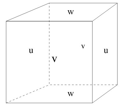
The Dimension Coordinates of the Arakawa C-Grid

Dimension coordinates have special meanings. The MITgcm uses the staggered Arakawa-C grid (hereafter c-grid). In c-grid models, variables are staggered in space. Horizontally, variables are associated with three ‘locations’:

1. tracer cells (e.g. temperature, salinity, density)

2. the 4 lateral faces of tracer cells (e.g., horizontal velocities and fluxes)

3. the 4 corners of tracer cells (e.g., vertical component of vorticity field)

Vertically, there are also two ‘locations’:

1. tracer cells

2. the 2 top/bottom faces of tracer cells (e.g., vertical velocities and fluxes).

To understand this better, let’s review the geometry of c-grid models.

3D staggering of velocity components.

Paraphrasing from https://mitgcm.readthedocs.io/en/latest/algorithm/c-grid.html,

In c-grid models, the components of flow (u,v,w) are staggered in
space such that the zonal component falls on the interface between
tracer cells in the zonal direction. Similarly for the meridional
and vertical directions.

Why the c-grid?

The basic algorithm employed for stepping forward the momentum
equations is based on retaining non-divergence of the flow at
all times. This is most naturally done if the components of flow
are staggered in space in the form of an Arakawa C grid...

Defining the c-grid coordinate system

As shown, variables on Arakawa-C grids (c-grid) are staggered in space. For convenience we define a coordinate system that distinguishes between these different locations.

The c-grid horizontal coordinates

In the horizontal, variables can take one of four locations: c, u, v, or g.

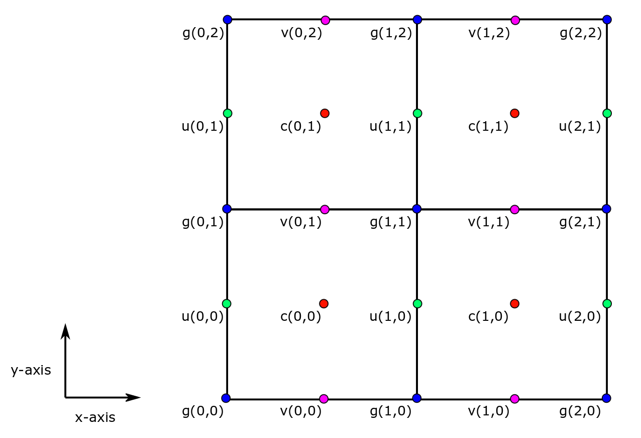
horizontal “c” location

Variables associated with tracer cell area or volumetric averages (e.g., temperature, salinity, sea ice thickness, air-sea net heat flux) and variables associated with vertical velocities (e.g., ) are identified with c locations.

For these variables we define the horizontal dimensions of i and j, corresponding with the model grid and directions, respectively.

horizontal “u” location

Variables associated with the two lateral sides of tracer cells in the direction are identified with u locations.

Define the horizontal dimensions of u variables as i_g and j, corresponding with the model’s and dimensions, respectively.

Important Note: In the llc90 curvilinear model grid used by ECCOv4, the direction is NOT same as the geographic zonal (east-west) direction.

horizontal “v” location

Variables associated with the two lateral sides of tracer cells in the direction are identified with v locations.

Define the horizontal dimensions of v variables as i and j_g, corresponding with the model’s and dimensions, respectively.

Important Note: In the llc90 curvilinear model grid used by ECCOv4, the direction is NOT same as the geographic meridional (north-south) direction.

horizontal “g” location

Variables associated with the horizontal corners of tracer grid cells are identified with g locations.

Define the horizontal dimensions of g variables as i_g and j_g, corresponding with the model’s and dimensions, respectively.

The c-grid vertical coordinates

In the horizontal, variables can take one of two locations: c and w

vertical “c” location

Variables associated with tracer cell volumetric quantities (e.g., temperature, salinity) are identified with c locations.

For these variables we define the vertical dimensions of k which corresponds with the model grid’ direction.

vertical “w” location

Variables associated with the two top/bottom sides of tracer cells in the direction are identified with w locations.

For these variables we define the vertical dimension of :math:`k_u` to indicate the model tracer cell’s upper faces in the direction, i.e., the bottom faces of the cell.

Two other vertical dimensions are also used. :math:`k_l` indicates the model tracer cell’s lower faces in the direction (i.e., the top faces of the cell), and which index all of the upper and lower faces.

Note: In ECCOv4 NetCDF files both :math:`k_l`(0) and :math:`k_{p1}`(0) correspond to the same top face of the model tracer grid cell.

All ECCOv4 coordinates

Now that we have been oriented to the dimensions and coordinates used by ECCOv4, let’s examine a Dataset that uses all of them, an ECCOv4r4 NetCDF grid file. The grid file for the native LLC90 grid has ShortName ECCO_L4_GEOMETRY_LLC0090GRID_V4R4. It does not have time dimensions, but we can put any StartDate and EndDate between 1992-01-01 and 2018-01-01 into the ecco_podaac_download function (or ecco_podaac_s3_get_diskaware function in the cloud) and it should retrieve the file. Then the file can be opened; in this case we’ll use open_dataset that loads a single file into memory in our workspace.

## download file containing grid parameters and load into workspace

ShortNames_list = ["ECCO_L4_GEOMETRY_LLC0090GRID_V4R4"]
if incloud_access == True:
    from ecco_s3_retrieve import ecco_podaac_s3_get_diskaware

    # retrieve file (download to instance if there is sufficient storage)
    files_nested_list = ecco_podaac_s3_get_diskaware(ShortNames=ShortNames_list,\
                                                     StartDate='2010-01',EndDate='2010-12',\
                                                     max_avail_frac=0.5,\
                                                     download_root_dir=ECCO_dir)

    # load file into workspace
    grid_dataset = xr.open_dataset(files_nested_list[ShortNames_list[0]])

else:
    from ecco_download import ecco_podaac_download

    # download grid file
    file_to_load = ecco_podaac_download(ShortName=grid_params_shortname,\
                   StartDate="2010-01-01",EndDate="2010-01-01",\
                   download_root_dir=ECCO_dir,n_workers=6,force_redownload=False)

    # load file into workspace
    grid_dataset = xr.open_dataset(files_to_load)

created download directory C:\Users\adelman\Downloads\ECCO_V4r4_PODAAC\ECCO_L4_GEOMETRY_LLC0090GRID_V4R4
{'ShortName': 'ECCO_L4_GEOMETRY_LLC0090GRID_V4R4', 'temporal': '2010-01-01,2010-01-01'}

Total number of matching granules: 1

100%|████████████████████████████████████████████████████████████████████████████████████| 1/1 [00:04<00:00,  4.37s/it]

=====================================
total downloaded: 8.57 Mb
avg download speed: 1.95 Mb/s

Open the ECCOv4r4 grid file:

# show contents of grid_dataset
grid_dataset

<xarray.Dataset> Size: 89MB
Dimensions:  (i: 90, i_g: 90, j: 90, j_g: 90, k: 50, k_u: 50, k_l: 50,
              k_p1: 51, tile: 13, nb: 4, nv: 2)
Coordinates: (12/20)
  * i        (i) int32 360B 0 1 2 3 4 5 6 7 8 9 ... 81 82 83 84 85 86 87 88 89
  * i_g      (i_g) int32 360B 0 1 2 3 4 5 6 7 8 9 ... 81 82 83 84 85 86 87 88 89
  * j        (j) int32 360B 0 1 2 3 4 5 6 7 8 9 ... 81 82 83 84 85 86 87 88 89
  * j_g      (j_g) int32 360B 0 1 2 3 4 5 6 7 8 9 ... 81 82 83 84 85 86 87 88 89
  * k        (k) int32 200B 0 1 2 3 4 5 6 7 8 9 ... 41 42 43 44 45 46 47 48 49
  * k_u      (k_u) int32 200B 0 1 2 3 4 5 6 7 8 9 ... 41 42 43 44 45 46 47 48 49
    ...       ...
    Zp1      (k_p1) float32 204B ...
    Zu       (k_u) float32 200B ...
    Zl       (k_l) float32 200B ...
    XC_bnds  (tile, j, i, nb) float32 2MB ...
    YC_bnds  (tile, j, i, nb) float32 2MB ...
    Z_bnds   (k, nv) float32 400B ...
Dimensions without coordinates: nb, nv
Data variables: (12/21)
    CS       (tile, j, i) float32 421kB ...
    SN       (tile, j, i) float32 421kB ...
    rA       (tile, j, i) float32 421kB ...
    dxG      (tile, j_g, i) float32 421kB ...
    dyG      (tile, j, i_g) float32 421kB ...
    Depth    (tile, j, i) float32 421kB ...
    ...       ...
    hFacC    (k, tile, j, i) float32 21MB ...
    hFacW    (k, tile, j, i_g) float32 21MB ...
    hFacS    (k, tile, j_g, i) float32 21MB ...
    maskC    (k, tile, j, i) bool 5MB ...
    maskW    (k, tile, j, i_g) bool 5MB ...
    maskS    (k, tile, j_g, i) bool 5MB ...
Attributes: (12/58)
    acknowledgement:                 This research was carried out by the Jet...
    author:                          Ian Fenty and Ou Wang
    cdm_data_type:                   Grid
    comment:                         Fields provided on the curvilinear lat-l...
    Conventions:                     CF-1.8, ACDD-1.3
    coordinates_comment:             Note: the global 'coordinates' attribute...
    ...                              ...
    references:                      ECCO Consortium, Fukumori, I., Wang, O.,...
    source:                          The ECCO V4r4 state estimate was produce...
    standard_name_vocabulary:        NetCDF Climate and Forecast (CF) Metadat...
    summary:                         This dataset provides geometric paramete...
    title:                           ECCO Geometry Parameters for the Lat-Lon...
    uuid:                            87ff7d24-86e5-11eb-9c5f-f8f21e2ee3e0

xarray.Dataset

• Dimensions:
  • i: 90
  • i_g: 90
  • j: 90
  • j_g: 90
  • k: 50
  • k_u: 50
  • k_l: 50
  • k_p1: 51
  • tile: 13
  • nb: 4
  • nv: 2
• Coordinates: (20)
  • i
    (i)
    int32
    0 1 2 3 4 5 6 ... 84 85 86 87 88 89

    axis :

    X

    long_name :

    grid index in x for variables at tracer and 'v' locations

    swap_dim :

    XC

    comment :

    In the Arakawa C-grid system, tracer (e.g., THETA) and 'v' variables (e.g., VVEL) have the same x coordinate on the model grid.

    coverage_content_type :

    coordinate

    array([ 0,  1,  2,  3,  4,  5,  6,  7,  8,  9, 10, 11, 12, 13, 14, 15, 16, 17,
           18, 19, 20, 21, 22, 23, 24, 25, 26, 27, 28, 29, 30, 31, 32, 33, 34, 35,
           36, 37, 38, 39, 40, 41, 42, 43, 44, 45, 46, 47, 48, 49, 50, 51, 52, 53,
           54, 55, 56, 57, 58, 59, 60, 61, 62, 63, 64, 65, 66, 67, 68, 69, 70, 71,
           72, 73, 74, 75, 76, 77, 78, 79, 80, 81, 82, 83, 84, 85, 86, 87, 88, 89],
          dtype=int32)

  • i_g
    (i_g)
    int32
    0 1 2 3 4 5 6 ... 84 85 86 87 88 89

    axis :

    X

    long_name :

    grid index in x for variables at 'u' and 'g' locations

    c_grid_axis_shift :

    -0.5

    swap_dim :

    XG

    comment :

    In the Arakawa C-grid system, 'u' (e.g., UVEL) and 'g' variables (e.g., XG) have the same x coordinate on the model grid.

    coverage_content_type :

    coordinate

    array([ 0,  1,  2,  3,  4,  5,  6,  7,  8,  9, 10, 11, 12, 13, 14, 15, 16, 17,
           18, 19, 20, 21, 22, 23, 24, 25, 26, 27, 28, 29, 30, 31, 32, 33, 34, 35,
           36, 37, 38, 39, 40, 41, 42, 43, 44, 45, 46, 47, 48, 49, 50, 51, 52, 53,
           54, 55, 56, 57, 58, 59, 60, 61, 62, 63, 64, 65, 66, 67, 68, 69, 70, 71,
           72, 73, 74, 75, 76, 77, 78, 79, 80, 81, 82, 83, 84, 85, 86, 87, 88, 89],
          dtype=int32)

  • j
    (j)
    int32
    0 1 2 3 4 5 6 ... 84 85 86 87 88 89

    axis :

    Y

    long_name :

    grid index in y for variables at tracer and 'u' locations

    swap_dim :

    YC

    comment :

    In the Arakawa C-grid system, tracer (e.g., THETA) and 'u' variables (e.g., UVEL) have the same y coordinate on the model grid.

    coverage_content_type :

    coordinate

    array([ 0,  1,  2,  3,  4,  5,  6,  7,  8,  9, 10, 11, 12, 13, 14, 15, 16, 17,
           18, 19, 20, 21, 22, 23, 24, 25, 26, 27, 28, 29, 30, 31, 32, 33, 34, 35,
           36, 37, 38, 39, 40, 41, 42, 43, 44, 45, 46, 47, 48, 49, 50, 51, 52, 53,
           54, 55, 56, 57, 58, 59, 60, 61, 62, 63, 64, 65, 66, 67, 68, 69, 70, 71,
           72, 73, 74, 75, 76, 77, 78, 79, 80, 81, 82, 83, 84, 85, 86, 87, 88, 89],
          dtype=int32)

  • j_g
    (j_g)
    int32
    0 1 2 3 4 5 6 ... 84 85 86 87 88 89

    axis :

    Y

    long_name :

    grid index in y for variables at 'v' and 'g' locations

    c_grid_axis_shift :

    -0.5

    swap_dim :

    YG

    comment :

    In the Arakawa C-grid system, 'v' (e.g., VVEL) and 'g' variables (e.g., XG) have the same y coordinate.

    coverage_content_type :

    coordinate

    array([ 0,  1,  2,  3,  4,  5,  6,  7,  8,  9, 10, 11, 12, 13, 14, 15, 16, 17,
           18, 19, 20, 21, 22, 23, 24, 25, 26, 27, 28, 29, 30, 31, 32, 33, 34, 35,
           36, 37, 38, 39, 40, 41, 42, 43, 44, 45, 46, 47, 48, 49, 50, 51, 52, 53,
           54, 55, 56, 57, 58, 59, 60, 61, 62, 63, 64, 65, 66, 67, 68, 69, 70, 71,
           72, 73, 74, 75, 76, 77, 78, 79, 80, 81, 82, 83, 84, 85, 86, 87, 88, 89],
          dtype=int32)

  • k
    (k)
    int32
    0 1 2 3 4 5 6 ... 44 45 46 47 48 49

    axis :

    Z

    long_name :

    grid index in z for tracer variables

    swap_dim :

    Z

    coverage_content_type :

    coordinate

    array([ 0,  1,  2,  3,  4,  5,  6,  7,  8,  9, 10, 11, 12, 13, 14, 15, 16, 17,
           18, 19, 20, 21, 22, 23, 24, 25, 26, 27, 28, 29, 30, 31, 32, 33, 34, 35,
           36, 37, 38, 39, 40, 41, 42, 43, 44, 45, 46, 47, 48, 49], dtype=int32)

  • k_u
    (k_u)
    int32
    0 1 2 3 4 5 6 ... 44 45 46 47 48 49

    axis :

    Z

    long_name :

    grid index in z corresponding to the bottom face of tracer grid cells ('w' locations)

    c_grid_axis_shift :

    0.5

    swap_dim :

    Zu

    comment :

    First index corresponds to the bottom face of the uppermost tracer grid cell. The use of 'u' in the variable name follows the MITgcm convention for naming the bottom face of ocean tracer grid cells.

    coverage_content_type :

    coordinate

    array([ 0,  1,  2,  3,  4,  5,  6,  7,  8,  9, 10, 11, 12, 13, 14, 15, 16, 17,
           18, 19, 20, 21, 22, 23, 24, 25, 26, 27, 28, 29, 30, 31, 32, 33, 34, 35,
           36, 37, 38, 39, 40, 41, 42, 43, 44, 45, 46, 47, 48, 49], dtype=int32)

  • k_l
    (k_l)
    int32
    0 1 2 3 4 5 6 ... 44 45 46 47 48 49

    axis :

    Z

    long_name :

    grid index in z corresponding to the top face of tracer grid cells ('w' locations)

    c_grid_axis_shift :

    -0.5

    swap_dim :

    Zl

    comment :

    First index corresponds to the top face of the uppermost tracer grid cell. The use of 'l' in the variable name follows the MITgcm convention for naming the top face of ocean tracer grid cells.

    coverage_content_type :

    coordinate

    array([ 0,  1,  2,  3,  4,  5,  6,  7,  8,  9, 10, 11, 12, 13, 14, 15, 16, 17,
           18, 19, 20, 21, 22, 23, 24, 25, 26, 27, 28, 29, 30, 31, 32, 33, 34, 35,
           36, 37, 38, 39, 40, 41, 42, 43, 44, 45, 46, 47, 48, 49], dtype=int32)

  • k_p1
    (k_p1)
    int32
    0 1 2 3 4 5 6 ... 45 46 47 48 49 50

    axis :

    Z

    long_name :

    grid index in z for variables at 'w' locations

    c_grid_axis_shift :

    [-0.5 0.5]

    swap_dim :

    Zp1

    comment :

    Includes top of uppermost model tracer cell (k_p1=0) and bottom of lowermost tracer cell (k_p1=51).

    coverage_content_type :

    coordinate

    array([ 0,  1,  2,  3,  4,  5,  6,  7,  8,  9, 10, 11, 12, 13, 14, 15, 16, 17,
           18, 19, 20, 21, 22, 23, 24, 25, 26, 27, 28, 29, 30, 31, 32, 33, 34, 35,
           36, 37, 38, 39, 40, 41, 42, 43, 44, 45, 46, 47, 48, 49, 50], dtype=int32)

  • tile
    (tile)
    int32
    0 1 2 3 4 5 6 7 8 9 10 11 12

    long_name :

    lat-lon-cap tile index

    comment :

    The ECCO V4 horizontal model grid is divided into 13 tiles of 90x90 cells for convenience.

    coverage_content_type :

    coordinate

    array([ 0,  1,  2,  3,  4,  5,  6,  7,  8,  9, 10, 11, 12], dtype=int32)

  • XC
    (tile, j, i)
    float32
    ...

    long_name :

    longitude of tracer grid cell center

    units :

    degrees_east

    coordinate :

    YC XC

    bounds :

    XC_bnds

    comment :

    nonuniform grid spacing

    coverage_content_type :

    coordinate

    standard_name :

    longitude

    [105300 values with dtype=float32]

  • YC
    (tile, j, i)
    float32
    ...

    long_name :

    latitude of tracer grid cell center

    units :

    degrees_north

    coordinate :

    YC XC

    bounds :

    YC_bnds

    comment :

    nonuniform grid spacing

    coverage_content_type :

    coordinate

    standard_name :

    latitude

    [105300 values with dtype=float32]

  • XG
    (tile, j_g, i_g)
    float32
    ...

    long_name :

    longitude of 'southwest' corner of tracer grid cell

    units :

    degrees_east

    coordinate :

    YG XG

    comment :

    Nonuniform grid spacing. Note: 'southwest' does not correspond to geographic orientation but is used for convenience to describe the computational grid. See MITgcm dcoumentation for details.

    coverage_content_type :

    coordinate

    standard_name :

    longitude

    [105300 values with dtype=float32]

  • YG
    (tile, j_g, i_g)
    float32
    ...

    long_name :

    latitude of 'southwest' corner of tracer grid cell

    units :

    degrees_north

    comment :

    Nonuniform grid spacing. Note: 'southwest' does not correspond to geographic orientation but is used for convenience to describe the computational grid. See MITgcm dcoumentation for details.

    coverage_content_type :

    coordinate

    standard_name :

    latitude

    [105300 values with dtype=float32]

  • Z
    (k)
    float32
    ...

    long_name :

    depth of tracer grid cell center

    units :

    m

    positive :

    up

    bounds :

    Z_bnds

    comment :

    Non-uniform vertical spacing.

    coverage_content_type :

    coordinate

    standard_name :

    depth

    [50 values with dtype=float32]

  • Zp1
    (k_p1)
    float32
    ...

    long_name :

    depth of top/bottom face of tracer grid cell

    units :

    m

    positive :

    up

    comment :

    Contains one element more than the number of vertical layers. First element is 0m, the depth of the top face of the uppermost grid cell. Last element is the depth of the bottom face of the deepest grid cell.

    coverage_content_type :

    coordinate

    standard_name :

    depth

    [51 values with dtype=float32]

  • Zu
    (k_u)
    float32
    ...

    long_name :

    depth of bottom face of tracer grid cell

    units :

    m

    positive :

    up

    comment :

    First element is -10m, the depth of the bottom face of the uppermost tracer grid cell. Last element is the depth of the bottom face of the deepest grid cell. The use of 'u' in the variable name follows the MITgcm convention for naming the bottom face of ocean tracer grid cells.

    coverage_content_type :

    coordinate

    standard_name :

    depth

    [50 values with dtype=float32]

  • Zl
    (k_l)
    float32
    ...

    long_name :

    depth of top face of tracer grid cell

    units :

    m

    positive :

    up

    comment :

    First element is 0m, the depth of the top face of the uppermost tracer grid cell (i.e., the ocean surface). Last element is the depth of the top face of the deepest grid cell. The use of 'l' in the variable name follows the MITgcm convention for naming the top face of ocean tracer grid cells.

    coverage_content_type :

    coordinate

    standard_name :

    depth

    [50 values with dtype=float32]

  • XC_bnds
    (tile, j, i, nb)
    float32
    ...

    comment :

    Bounds array follows CF conventions. XC_bnds[i,j,0] = 'southwest' corner (j-1, i-1), XC_bnds[i,j,1] = 'southeast' corner (j-1, i+1), XC_bnds[i,j,2] = 'northeast' corner (j+1, i+1), XC_bnds[i,j,3] = 'northwest' corner (j+1, i-1). Note: 'southwest', 'southeast', northwest', and 'northeast' do not correspond to geographic orientation but are used for convenience to describe the computational grid. See MITgcm dcoumentation for details.

    coverage_content_type :

    coordinate

    long_name :

    longitudes of tracer grid cell corners

    [421200 values with dtype=float32]

  • YC_bnds
    (tile, j, i, nb)
    float32
    ...

    comment :

    Bounds array follows CF conventions. YC_bnds[i,j,0] = 'southwest' corner (j-1, i-1), YC_bnds[i,j,1] = 'southeast' corner (j-1, i+1), YC_bnds[i,j,2] = 'northeast' corner (j+1, i+1), YC_bnds[i,j,3] = 'northwest' corner (j+1, i-1). Note: 'southwest', 'southeast', northwest', and 'northeast' do not correspond to geographic orientation but are used for convenience to describe the computational grid. See MITgcm dcoumentation for details.

    coverage_content_type :

    coordinate

    long_name :

    latitudes of tracer grid cell corners

    [421200 values with dtype=float32]

  • Z_bnds
    (k, nv)
    float32
    ...

    comment :

    One pair of depths for each vertical level.

    coverage_content_type :

    coordinate

    long_name :

    depths of top and bottom faces of tracer grid cell

    [100 values with dtype=float32]

• Data variables: (21)
  • CS
    (tile, j, i)
    float32
    ...

    long_name :

    cosine of tracer grid cell orientation vs geographical north

    units :

    1

    coordinate :

    YC XC

    coverage_content_type :

    modelResult

    comment :

    CS and SN are required to calculate the geographic (meridional, zonal) components of vectors on the curvilinear model grid. Note: for vector R with components R_x and R_y: R_{east} = CS R_x - SN R_y. R_{north} = SN R_x + CS R_y

    [105300 values with dtype=float32]

  • SN
    (tile, j, i)
    float32
    ...

    long_name :

    sine of tracer grid cell orientation vs geographical north

    units :

    1

    coordinate :

    YC XC

    coverage_content_type :

    modelResult

    comment :

    CS and SN are required to calculate the geographic (meridional, zonal) components of vectors on the curvilinear model grid. Note: for vector R with components R_x and R_y in local grid directions x and y, the geographical eastward component R_{east} = CS R_x - SN R_y. The geographical northward component R_{north} = SN R_x + CS R_y.

    [105300 values with dtype=float32]

  • rA
    (tile, j, i)
    float32
    ...

    long_name :

    area of tracer grid cell

    units :

    m2

    coordinate :

    YC XC

    coverage_content_type :

    modelResult

    standard_name :

    cell_area

    [105300 values with dtype=float32]

  • dxG
    (tile, j_g, i)
    float32
    ...

    long_name :

    distance between 'southwest' and 'southeast' corners of the tracer grid cell

    units :

    m

    coordinate :

    YG XC

    coverage_content_type :

    modelResult

    comment :

    Alternatively, the length of 'south' side of tracer grid cell. Note: 'south', 'southwest', and 'southeast' do not correspond to geographic orientation but are used for convenience to describe the computational grid. See MITgcm documentation for details.

    [105300 values with dtype=float32]

  • dyG
    (tile, j, i_g)
    float32
    ...

    long_name :

    distance between 'southwest' and 'northwest' corners of the tracer grid cell

    units :

    m

    coordinate :

    YC XG

    coverage_content_type :

    modelResult

    comment :

    Alternatively, the length of 'west' side of tracer grid cell. Note: 'west, 'southwest', and 'northwest' do not correspond to geographic orientation but are used for convenience to describe the computational grid. See MITgcm documentation for details.

    [105300 values with dtype=float32]

  • Depth
    (tile, j, i)
    float32
    ...

    long_name :

    model seafloor depth below ocean surface at rest

    units :

    m

    coordinate :

    XC YC

    coverage_content_type :

    modelResult

    standard_name :

    sea_floor_depth_below_geoid

    comment :

    Model sea surface height (SSH) of 0m corresponds to an ocean surface at rest relative to the geoid. Depth corresponds to seafloor depth below geoid. Note: the MITgcm used by ECCO V4r4 implements 'partial cells' so the actual model seafloor depth may differ from the seafloor depth provided by the input bathymetry file.

    [105300 values with dtype=float32]

  • rAz
    (tile, j_g, i_g)
    float32
    ...

    long_name :

    area of vorticity 'g' grid cell

    units :

    m2

    coordinate :

    YG XG

    coverage_content_type :

    modelResult

    standard_name :

    cell_area

    comment :

    Vorticity cells are staggered in space relative to tracer cells, nominally situated on tracer cell corners. Vorticity cell (i,j) is located at the 'southwest' corner of tracer grid cell (i, j). Note: 'southwest' does not correspond to geographic orientation but is used for convenience to describe the computational grid. See MITgcm documentation for details.

    [105300 values with dtype=float32]

  • dxC
    (tile, j, i_g)
    float32
    ...

    long_name :

    distance between centers of adjacent tracer grid cells in the 'x' direction

    units :

    m

    coordinate :

    YC XG

    coverage_content_type :

    modelResult

    comment :

    Alternatively, the length of 'north' side of vorticity grid cells. Note: 'north' does not correspond to geographic orientation but is used for convenience to describe the computational grid. See MITgcm documentation for details.

    [105300 values with dtype=float32]

  • dyC
    (tile, j_g, i)
    float32
    ...

    long_name :

    distance between centers of adjacent tracer grid cells in the 'y' direction

    units :

    m

    coordinate :

    YG XC

    coverage_content_type :

    modelResult

    comment :

    Alternatively, the length of 'east' side of vorticity grid cells. Note: 'east' does not correspond to geographic orientation but is used for convenience to describe the computational grid. See MITgcm documentation for details.

    [105300 values with dtype=float32]

  • rAw
    (tile, j, i_g)
    float32
    ...

    long_name :

    area of 'v' grid cell

    units :

    m2

    coordinate :

    YG XC

    coverage_content_type :

    modelResult

    standard_name :

    cell_area

    comment :

    Model 'v' grid cells are staggered in space between adjacent tracer grid cells in the 'x' direction. 'v' grid cell (i,j) is situated at the 'west' edge of tracer grid cell (i, j). Note: 'west' does not correspond to geographic orientation but is used for convenience to describe the computational grid. See MITgcm documentation for details.

    [105300 values with dtype=float32]

  • rAs
    (tile, j_g, i)
    float32
    ...

    long_name :

    area of 'u' grid cell

    units :

    m2

    coverage_content_type :

    modelResult

    standard_name :

    cell_area

    comment :

    Model 'u' grid cells are staggered in space between adjacent tracer grid cells in the 'y' direction. 'u' grid cell (i,j) is situated at the 'south' edge of tracer grid cell (i, j). Note: 'south' does not correspond to geographic orientation but is used for convenience to describe the computational grid. See MITgcm documentation for details.

    [105300 values with dtype=float32]

  • drC
    (k_p1)
    float32
    ...

    long_name :

    distance between the centers of adjacent tracer grid cells in the 'z' direction

    units :

    m

    coverage_content_type :

    modelResult

    comment :

    The first element corresponds to the distance between the depth of the center of the uppermost model grid cell and the surface.

    [51 values with dtype=float32]

  • drF
    (k)
    float32
    ...

    long_name :

    distance between the upper and lower interfaces of the model grid cell

    units :

    m

    coverage_content_type :

    modelResult

    standard_name :

    cell_thickness

    comment :

    Nominal grid cell thickness. Note: in the z* coordinate system used in ECCO V4, actual tracer grid cell thickness, h, varies through time as h(i,j,k,t)= drF(k) hfacC(i,j,k,t).

    [50 values with dtype=float32]

  • PHrefC
    (k)
    float32
    ...

    long_name :

    reference ocean hydrostatic pressure at tracer grid cell center

    units :

    m2 s-2

    coverage_content_type :

    modelResult

    comment :

    PHrefC = p_ref (k) / rhoConst = rhoConst g z(k) / rhoConst = g z(k), where p_ref(k) is reference hydrostatic ocean pressure at center of tracer grid cell k, rhoConst is reference density (1029 kg m-3), g is acceleration due to gravity (9.81 m s-2), and z(k) is depth at center of tracer grid cell k. Units: p:[kg m-1 s-2], rhoConst:[kg m-3], g:[m s-2], z_m(t):[m]. Note: does not include atmospheric pressure loading. Quantity referred to in some contexts as hydrostatic pressure potential. PHIHYDcR is anomaly of PHrefC.

    [50 values with dtype=float32]

  • PHrefF
    (k_p1)
    float32
    ...

    long_name :

    reference ocean hydrostatic pressure at tracer grid cell top/bottom interface

    units :

    m2 s-2

    coverage_content_type :

    modelResult

    comment :

    PHrefF = p_ref (k_l) / rhoConst = rhoConst g z(k_l) / rhoConst = g z(k_l), where p_ref(k_l) is reference hydrostatic ocean pressure at lower interface of tracer grid cell k, rhoConst is reference density (1029 kg m-3), g is acceleration due to gravity (9.81 m s-2), and z(k) is depth at center of tracer grid cell k. Units: p:[kg m-1 s-2], rhoConst:[kg m-3], g:[m s-2], z_m(t):[m]. Note: does not include atmospheric pressure loading. Quantity referred to in some contexts as hydrostatic pressure potential. See PHrefC

    [51 values with dtype=float32]

  • hFacC
    (k, tile, j, i)
    float32
    ...

    long_name :

    vertical open fraction of tracer grid cell

    coverage_content_type :

    modelResult

    units :

    1

    comment :

    Tracer grid cells may be fractionally closed in the vertical. The open vertical fraction is hFacC. The model allows for partially-filled cells to represent topographic variations more smoothly (hFacC < 1). Completely closed (dry) tracer grid cells have hFacC = 0. Note: the model z* coordinate system allows hFacC to vary through time. A time-invariant hFacC field is provided for reference.

    [5265000 values with dtype=float32]

  • hFacW
    (k, tile, j, i_g)
    float32
    ...

    long_name :

    vertical open fraction of tracer grid cell 'west' face

    coverage_content_type :

    modelResult

    units :

    1

    comment :

    The 'west' face of tracer grid cells may be fractionally closed in the vertical. The open vertical fraction is hFacW. The model allows for partially-filled cells for smoother representation of seafloor topography. Tracer grid cells adjacent in the 'x' direction that are partially closed in the vertical have hFacW < 1. The model z* coordinate system used by the model permits hFacC, and therefore hFacW, to vary through time. A time-invariant hFacW field is provided for reference. Note: The term 'west' does not correspond to geographic orientation but is used for convenience to describe the computational grid. See MITgcm documentation for details.

    [5265000 values with dtype=float32]

  • hFacS
    (k, tile, j_g, i)
    float32
    ...

    long_name :

    vertical open fraction of tracer grid cell 'south' face

    coverage_content_type :

    modelResult

    units :

    1

    comment :

    The 'south' face of tracer grid cells may be fractionally closed in the vertical. The open vertical fraction is hFacS. The model allows for partially-filled cells for smoother representation of seafloor topography. Tracer grid cells adjacent in the 'y' direction that are partially closed in the vertical have hFacS < 1. The model z* coordinate system used by the model permits hFacC, and therefore hFacS, to vary through time. A time-invariant hFacS field is provided for reference. Note: The term 'south' does not correspond to geographic orientation but is used for convenience to describe the computational grid. See MITgcm documentation for details.

    [5265000 values with dtype=float32]

  • maskC
    (k, tile, j, i)
    bool
    ...

    long_name :

    wet/dry boolean mask for tracer grid cell

    coverage_content_type :

    modelResult

    comment :

    True for tracer grid cells with nonzero open vertical fraction (hFacC > 0), otherwise False. Although hFacC can vary though time, cells will never close if starting open and will never open if starting closed: hFacC(i,j,k,t) > 0 for all t, if hFacC(i,j,k,t=0) and hFacC(i,j,k,t) = 0 for all t, if hFacC(i,j,k,t=0) = 0. Therefore, maskC is time invariant.

    [5265000 values with dtype=bool]

  • maskW
    (k, tile, j, i_g)
    bool
    ...

    long_name :

    wet/dry boolean mask for 'west' face of tracer grid cell

    coverage_content_type :

    modelResult

    comment :

    True for grid cells with nonzero open vertical fraction along their 'west' face (hFacW > 0), otherwise False. Although hFacW can vary though time, cells will never close if starting open and will never open if starting closed: hFacW(i,j,k,t) > 0 for all t, if hFacW(i,j,k,t=0) and hFacW(i,j,k,t) = 0 for all t, if hFacW(i,j,k,t=0) = 0. Therefore, maskW is time invariant. Note:

    [5265000 values with dtype=bool]

  • maskS
    (k, tile, j_g, i)
    bool
    ...

    long_name :

    wet/dry boolean mask for 'south' face of tracer grid cell

    coverage_content_type :

    modelResult

    comment :

    True for grid cells with nonzero open vertical fraction along their 'south' face (hFacS > 0), otherwise False. Although hFacS can vary though time, cells will never close if starting open and will never open if starting closed: hFacS(i,j,k,t) > 0 for all t, if hFacS(i,j,k,t=0) and hFacS(i,j,k,t) = 0 for all t, if hFacS(i,j,k,t=0) = 0. Therefore, maskS is time invariant. Note:

    [5265000 values with dtype=bool]

• Indexes: (9)
  • i
    PandasIndex

    PandasIndex(Index([ 0,  1,  2,  3,  4,  5,  6,  7,  8,  9, 10, 11, 12, 13, 14, 15, 16, 17,
           18, 19, 20, 21, 22, 23, 24, 25, 26, 27, 28, 29, 30, 31, 32, 33, 34, 35,
           36, 37, 38, 39, 40, 41, 42, 43, 44, 45, 46, 47, 48, 49, 50, 51, 52, 53,
           54, 55, 56, 57, 58, 59, 60, 61, 62, 63, 64, 65, 66, 67, 68, 69, 70, 71,
           72, 73, 74, 75, 76, 77, 78, 79, 80, 81, 82, 83, 84, 85, 86, 87, 88, 89],
          dtype='int32', name='i'))

  • i_g
    PandasIndex

    PandasIndex(Index([ 0,  1,  2,  3,  4,  5,  6,  7,  8,  9, 10, 11, 12, 13, 14, 15, 16, 17,
           18, 19, 20, 21, 22, 23, 24, 25, 26, 27, 28, 29, 30, 31, 32, 33, 34, 35,
           36, 37, 38, 39, 40, 41, 42, 43, 44, 45, 46, 47, 48, 49, 50, 51, 52, 53,
           54, 55, 56, 57, 58, 59, 60, 61, 62, 63, 64, 65, 66, 67, 68, 69, 70, 71,
           72, 73, 74, 75, 76, 77, 78, 79, 80, 81, 82, 83, 84, 85, 86, 87, 88, 89],
          dtype='int32', name='i_g'))

  • j
    PandasIndex

    PandasIndex(Index([ 0,  1,  2,  3,  4,  5,  6,  7,  8,  9, 10, 11, 12, 13, 14, 15, 16, 17,
           18, 19, 20, 21, 22, 23, 24, 25, 26, 27, 28, 29, 30, 31, 32, 33, 34, 35,
           36, 37, 38, 39, 40, 41, 42, 43, 44, 45, 46, 47, 48, 49, 50, 51, 52, 53,
           54, 55, 56, 57, 58, 59, 60, 61, 62, 63, 64, 65, 66, 67, 68, 69, 70, 71,
           72, 73, 74, 75, 76, 77, 78, 79, 80, 81, 82, 83, 84, 85, 86, 87, 88, 89],
          dtype='int32', name='j'))

  • j_g
    PandasIndex

    PandasIndex(Index([ 0,  1,  2,  3,  4,  5,  6,  7,  8,  9, 10, 11, 12, 13, 14, 15, 16, 17,
           18, 19, 20, 21, 22, 23, 24, 25, 26, 27, 28, 29, 30, 31, 32, 33, 34, 35,
           36, 37, 38, 39, 40, 41, 42, 43, 44, 45, 46, 47, 48, 49, 50, 51, 52, 53,
           54, 55, 56, 57, 58, 59, 60, 61, 62, 63, 64, 65, 66, 67, 68, 69, 70, 71,
           72, 73, 74, 75, 76, 77, 78, 79, 80, 81, 82, 83, 84, 85, 86, 87, 88, 89],
          dtype='int32', name='j_g'))

  • k
    PandasIndex

    PandasIndex(Index([ 0,  1,  2,  3,  4,  5,  6,  7,  8,  9, 10, 11, 12, 13, 14, 15, 16, 17,
           18, 19, 20, 21, 22, 23, 24, 25, 26, 27, 28, 29, 30, 31, 32, 33, 34, 35,
           36, 37, 38, 39, 40, 41, 42, 43, 44, 45, 46, 47, 48, 49],
          dtype='int32', name='k'))

  • k_u
    PandasIndex

    PandasIndex(Index([ 0,  1,  2,  3,  4,  5,  6,  7,  8,  9, 10, 11, 12, 13, 14, 15, 16, 17,
           18, 19, 20, 21, 22, 23, 24, 25, 26, 27, 28, 29, 30, 31, 32, 33, 34, 35,
           36, 37, 38, 39, 40, 41, 42, 43, 44, 45, 46, 47, 48, 49],
          dtype='int32', name='k_u'))

  • k_l
    PandasIndex

    PandasIndex(Index([ 0,  1,  2,  3,  4,  5,  6,  7,  8,  9, 10, 11, 12, 13, 14, 15, 16, 17,
           18, 19, 20, 21, 22, 23, 24, 25, 26, 27, 28, 29, 30, 31, 32, 33, 34, 35,
           36, 37, 38, 39, 40, 41, 42, 43, 44, 45, 46, 47, 48, 49],
          dtype='int32', name='k_l'))

  • k_p1
    PandasIndex

    PandasIndex(Index([ 0,  1,  2,  3,  4,  5,  6,  7,  8,  9, 10, 11, 12, 13, 14, 15, 16, 17,
           18, 19, 20, 21, 22, 23, 24, 25, 26, 27, 28, 29, 30, 31, 32, 33, 34, 35,
           36, 37, 38, 39, 40, 41, 42, 43, 44, 45, 46, 47, 48, 49, 50],
          dtype='int32', name='k_p1'))

  • tile
    PandasIndex

    PandasIndex(Index([0, 1, 2, 3, 4, 5, 6, 7, 8, 9, 10, 11, 12], dtype='int32', name='tile'))

• Attributes: (58)

  acknowledgement :

  This research was carried out by the Jet Propulsion Laboratory, managed by the California Institute of Technology under a contract with the National Aeronautics and Space Administration.

  author :

  Ian Fenty and Ou Wang

  cdm_data_type :

  Grid

  comment :

  Fields provided on the curvilinear lat-lon-cap 90 (llc90) native grid used in the ECCO model.

  Conventions :

  CF-1.8, ACDD-1.3

  coordinates_comment :

  Note: the global 'coordinates' attribute describes auxillary coordinates.

  creator_email :

  ecco-group@mit.edu

  creator_institution :

  NASA Jet Propulsion Laboratory (JPL)

  creator_name :

  ECCO Consortium

  creator_type :

  group

  creator_url :

  https://ecco-group.org

  date_created :

  2021-03-16T22:56:35

  date_issued :

  2021-03-16T22:56:35

  date_metadata_modified :

  2021-03-16T22:56:35

  date_modified :

  2021-03-16T22:56:35

  geospatial_bounds_crs :

  EPSG:4326

  geospatial_lat_max :

  90.0

  geospatial_lat_min :

  -90.0

  geospatial_lat_resolution :

  variable

  geospatial_lat_units :

  degrees_north

  geospatial_lon_max :

  180.0

  geospatial_lon_min :

  -180.0

  geospatial_lon_resolution :

  variable

  geospatial_lon_units :

  degrees_east

  geospatial_vertical_max :

  0.0

  geospatial_vertical_min :

  -6134.5

  geospatial_vertical_positive :

  up

  geospatial_vertical_resolution :

  variable

  geospatial_vertical_units :

  meter

  history :

  Inaugural release of an ECCO Central Estimate solution to PO.DAAC

  id :

  10.5067/ECL5A-GRD44

  institution :

  NASA Jet Propulsion Laboratory (JPL)

  instrument_vocabulary :

  GCMD instrument keywords

  keywords :

  EARTH SCIENCE SERVICES > MODELS > EARTH SCIENCE REANALYSES/ASSIMILATION MODELS

  keywords_vocabulary :

  NASA Global Change Master Directory (GCMD) Science Keywords

  license :

  Public Domain

  metadata_link :

  https://cmr.earthdata.nasa.gov/search/collections.umm_json?ShortName=ECCO_L4_GEOMETRY_LLC0090GRID_V4R4

  naming_authority :

  gov.nasa.jpl

  platform :

  ERS-1/2, TOPEX/Poseidon, Geosat Follow-On (GFO), ENVISAT, Jason-1, Jason-2, CryoSat-2, SARAL/AltiKa, Jason-3, AVHRR, Aquarius, SSM/I, SSMIS, GRACE, DTU17MDT, Argo, WOCE, GO-SHIP, MEOP, Ice Tethered Profilers (ITP)

  platform_vocabulary :

  GCMD platform keywords

  processing_level :

  L4

  product_name :

  GRID_GEOMETRY_ECCO_V4r4_native_llc0090.nc

  product_time_coverage_end :

  2018-01-01T00:00:00

  product_time_coverage_start :

  1992-01-01T12:00:00

  product_version :

  Version 4, Release 4

  program :

  NASA Physical Oceanography, Cryosphere, Modeling, Analysis, and Prediction (MAP)

  project :

  Estimating the Circulation and Climate of the Ocean (ECCO)

  publisher_email :

  podaac@podaac.jpl.nasa.gov

  publisher_institution :

  PO.DAAC

  publisher_name :

  Physical Oceanography Distributed Active Archive Center (PO.DAAC)

  publisher_type :

  institution

  publisher_url :

  https://podaac.jpl.nasa.gov

  references :

  ECCO Consortium, Fukumori, I., Wang, O., Fenty, I., Forget, G., Heimbach, P., & Ponte, R. M. 2020. Synopsis of the ECCO Central Production Global Ocean and Sea-Ice State Estimate (Version 4 Release 4). doi:10.5281/zenodo.3765928

  source :

  The ECCO V4r4 state estimate was produced by fitting a free-running solution of the MITgcm (checkpoint 66g) to satellite and in situ observational data in a least squares sense using the adjoint method

  standard_name_vocabulary :

  NetCDF Climate and Forecast (CF) Metadata Convention

  summary :

  This dataset provides geometric parameters for the lat-lon-cap 90 (llc90) native model grid from the ECCO Version 4 Release 4 (V4r4) ocean and sea-ice state estimate. Parameters include areas and lengths of grid cell sides, horizontal and vertical coordinates of grid cell centers and corners, grid rotation angles, and global domain geometry including bathymetry and land/ocean masks. Estimating the Circulation and Climate of the Ocean (ECCO) state estimates are dynamically and kinematically-consistent reconstructions of the three-dimensional, time-evolving ocean, sea-ice, and surface atmospheric states. ECCO V4r4 is a free-running solution of a global, nominally 1-degree configuration of the MIT general circulation model (MITgcm) that has been fit to observations in a least-squares sense. Observational data constraints used in V4r4 include sea surface height (SSH) from satellite altimeters [ERS-1/2, TOPEX/Poseidon, GFO, ENVISAT, Jason-1,2,3, CryoSat-2, and SARAL/AltiKa]; sea surface temperature (SST) from satellite radiometers [AVHRR], sea surface salinity (SSS) from the Aquarius satellite radiometer/scatterometer, ocean bottom pressure (OBP) from the GRACE satellite gravimeter; sea-ice concentration from satellite radiometers [SSM/I and SSMIS], and in-situ ocean temperature and salinity measured with conductivity-temperature-depth (CTD) sensors and expendable bathythermographs (XBTs) from several programs [e.g., WOCE, GO-SHIP, Argo, and others] and platforms [e.g., research vessels, gliders, moorings, ice-tethered profilers, and instrumented pinnipeds]. V4r4 covers the period 1992-01-01T12:00:00 to 2018-01-01T00:00:00.

  title :

  ECCO Geometry Parameters for the Lat-Lon-Cap 90 (llc90) Native Model Grid (Version 4 Release 4)

  uuid :

  87ff7d24-86e5-11eb-9c5f-f8f21e2ee3e0

You’ll notice that the dimensions and coordinates of the grid file are the same as for the potential temperature/salinity files we looked at before, except that there is no time dimension or time-related coordinates. Let’s move on to the Data variables, which in this file are parameters associated with the grid.

Grid Parameters

There are 21 data variables in the grid file. These grid parameters describe the model grid geometry, and are essential for quantitative analysis with ECCO output.

axis rotation factors:

CS       (tile, j, i)   float32 ...
SN       (tile, j, i)   float32 ...

horizontal distances:

dxG      (tile, j_g, i) float32 ...
dyG      (tile, j, i_g) float32 ...
dxC      (tile, j, i_g) float32 ...
dyC      (tile, j_g, i) float32 ...

vertical distances:

drC      (k_p1) float32 ...
drF      (k) float32 ...

areas:

rA       (tile, j, i) float32 ...
rAz      (tile, j_g, i_g) float32 ...
rAw      (tile, j, i_g) float32 ...
rAs      (tile, j_g, i) float32 ...

reference hydrostatic pressure at cell depth:

PHrefC   (k) float32 ...
PHrefF   (k_p1) float32 ...

partial cell fractions:

hFacC    (k, tile, j, i) float32 ...
hFacW    (k, tile, j, i_g) float32 ...
hFacS    (k, tile, j_g, i) float32 ...

wet/dry boolean masks:

maskC    (k, tile, j, i) bool ...
maskW    (k, tile, j, i_g) bool ...
maskS    (k, tile, j_g, i) bool ...

seafloor depth:

Depth    (j, i) float32 ...

Grid parameters are not coordinates in the sense that they help you orient in space or time, but they provide measures of the model grid such as distances and areas. Let’s examine one of these grid geometric variables, dxG:

grid_dataset.dxG

<xarray.DataArray 'dxG' (tile: 13, j_g: 90, i: 90)> Size: 421kB
[105300 values with dtype=float32]
Coordinates:
  * i        (i) int32 360B 0 1 2 3 4 5 6 7 8 9 ... 81 82 83 84 85 86 87 88 89
  * j_g      (j_g) int32 360B 0 1 2 3 4 5 6 7 8 9 ... 81 82 83 84 85 86 87 88 89
  * tile     (tile) int32 52B 0 1 2 3 4 5 6 7 8 9 10 11 12
Attributes:
    long_name:              distance between 'southwest' and 'southeast' corn...
    units:                  m
    coordinate:             YG XC
    coverage_content_type:  modelResult
    comment:                Alternatively, the length of 'south' side of trac...

xarray.DataArray

'dxG'

• tile: 13
• j_g: 90
• i: 90

• ...

  [105300 values with dtype=float32]

• Coordinates: (3)
  • i
    (i)
    int32
    0 1 2 3 4 5 6 ... 84 85 86 87 88 89

    axis :

    X

    long_name :

    grid index in x for variables at tracer and 'v' locations

    swap_dim :

    XC

    comment :

    In the Arakawa C-grid system, tracer (e.g., THETA) and 'v' variables (e.g., VVEL) have the same x coordinate on the model grid.

    coverage_content_type :

    coordinate

    array([ 0,  1,  2,  3,  4,  5,  6,  7,  8,  9, 10, 11, 12, 13, 14, 15, 16, 17,
           18, 19, 20, 21, 22, 23, 24, 25, 26, 27, 28, 29, 30, 31, 32, 33, 34, 35,
           36, 37, 38, 39, 40, 41, 42, 43, 44, 45, 46, 47, 48, 49, 50, 51, 52, 53,
           54, 55, 56, 57, 58, 59, 60, 61, 62, 63, 64, 65, 66, 67, 68, 69, 70, 71,
           72, 73, 74, 75, 76, 77, 78, 79, 80, 81, 82, 83, 84, 85, 86, 87, 88, 89],
          dtype=int32)

  • j_g
    (j_g)
    int32
    0 1 2 3 4 5 6 ... 84 85 86 87 88 89

    axis :

    Y

    long_name :

    grid index in y for variables at 'v' and 'g' locations

    c_grid_axis_shift :

    -0.5

    swap_dim :

    YG

    comment :

    In the Arakawa C-grid system, 'v' (e.g., VVEL) and 'g' variables (e.g., XG) have the same y coordinate.

    coverage_content_type :

    coordinate

    array([ 0,  1,  2,  3,  4,  5,  6,  7,  8,  9, 10, 11, 12, 13, 14, 15, 16, 17,
           18, 19, 20, 21, 22, 23, 24, 25, 26, 27, 28, 29, 30, 31, 32, 33, 34, 35,
           36, 37, 38, 39, 40, 41, 42, 43, 44, 45, 46, 47, 48, 49, 50, 51, 52, 53,
           54, 55, 56, 57, 58, 59, 60, 61, 62, 63, 64, 65, 66, 67, 68, 69, 70, 71,
           72, 73, 74, 75, 76, 77, 78, 79, 80, 81, 82, 83, 84, 85, 86, 87, 88, 89],
          dtype=int32)

  • tile
    (tile)
    int32
    0 1 2 3 4 5 6 7 8 9 10 11 12

    long_name :

    lat-lon-cap tile index

    comment :

    The ECCO V4 horizontal model grid is divided into 13 tiles of 90x90 cells for convenience.

    coverage_content_type :

    coordinate

    array([ 0,  1,  2,  3,  4,  5,  6,  7,  8,  9, 10, 11, 12], dtype=int32)

• Indexes: (3)
  • i
    PandasIndex

    PandasIndex(Index([ 0,  1,  2,  3,  4,  5,  6,  7,  8,  9, 10, 11, 12, 13, 14, 15, 16, 17,
           18, 19, 20, 21, 22, 23, 24, 25, 26, 27, 28, 29, 30, 31, 32, 33, 34, 35,
           36, 37, 38, 39, 40, 41, 42, 43, 44, 45, 46, 47, 48, 49, 50, 51, 52, 53,
           54, 55, 56, 57, 58, 59, 60, 61, 62, 63, 64, 65, 66, 67, 68, 69, 70, 71,
           72, 73, 74, 75, 76, 77, 78, 79, 80, 81, 82, 83, 84, 85, 86, 87, 88, 89],
          dtype='int32', name='i'))

  • j_g
    PandasIndex

    PandasIndex(Index([ 0,  1,  2,  3,  4,  5,  6,  7,  8,  9, 10, 11, 12, 13, 14, 15, 16, 17,
           18, 19, 20, 21, 22, 23, 24, 25, 26, 27, 28, 29, 30, 31, 32, 33, 34, 35,
           36, 37, 38, 39, 40, 41, 42, 43, 44, 45, 46, 47, 48, 49, 50, 51, 52, 53,
           54, 55, 56, 57, 58, 59, 60, 61, 62, 63, 64, 65, 66, 67, 68, 69, 70, 71,
           72, 73, 74, 75, 76, 77, 78, 79, 80, 81, 82, 83, 84, 85, 86, 87, 88, 89],
          dtype='int32', name='j_g'))

  • tile
    PandasIndex

    PandasIndex(Index([0, 1, 2, 3, 4, 5, 6, 7, 8, 9, 10, 11, 12], dtype='int32', name='tile'))

• Attributes: (5)

  long_name :

  distance between 'southwest' and 'southeast' corners of the tracer grid cell

  units :

  m

  coordinate :

  YG XC

  coverage_content_type :

  modelResult

  comment :

  Alternatively, the length of 'south' side of tracer grid cell. Note: 'south', 'southwest', and 'southeast' do not correspond to geographic orientation but are used for convenience to describe the computational grid. See MITgcm documentation for details.

dxG has coordinates tile, j_g and i which means that it is a v location variable. dxG is the horizontal distance between points (tracer cell corners) in the tile’s direction.

For reference, see the chart below from the MITgcm documentation, Figure 2.6

dxG = in subfigure (a) below:

Figure 2.6 Staggering of horizontal grid descriptors (lengths and areas). The grid lines indicate the tracer cell boundaries and are the reference grid for all panels. a) The area of a tracer cell, 𝐴𝑐, is bordered by the lengths Δ𝑥𝑔 and Δ𝑦𝑔. b) The area of a vorticity cell, 𝐴𝜁, is bordered by the lengths Δ𝑥𝑐 and Δ𝑦𝑐. c) The area of a u cell, 𝐴𝑤, is bordered by the lengths Δ𝑥𝑣 and Δ𝑦𝑓. d) The area of a v cell, 𝐴𝑠, is bordered by the lengths Δ𝑥𝑓 and Δ𝑦𝑢.

Dimensions and Coordinates of Velocities

So far we looked at files with THETA and SALT which are variables (i.e. tracers). Let’s examine UVEL, horizontal velocity in the tile’s direction. As you’ve probably guessed, UVEL is a variable:

Let’s download and open the March 2010 mean horizontal velocity.

## download file containing monthly mean ocean velocities for March 2010, and load into workspace

ShortNames_list = ["ECCO_L4_OCEAN_VEL_LLC0090GRID_MONTHLY_V4R4"]
if incloud_access == True:
    # retrieve file (download to instance if there is sufficient storage)
    files_nested_list = ecco_podaac_s3_get_diskaware(ShortNames=ShortNames_list,\
                                                     StartDate='2010-03',EndDate='2010-03',\
                                                     max_avail_frac=0.5,\
                                                     download_root_dir=ECCO_dir)

    # load file into workspace
    vel_dataset = xr.open_dataset(files_nested_list[ShortNames_list[0]])

else:
    # download velocity file
    file_to_load = ecco_podaac_download(ShortName=vel_shortname,\
                                        StartDate='2010-03',EndDate='2010-03',\
                                        download_root_dir=ECCO_dir,n_workers=6,force_redownload=False)

    # load file into workspace
    vel_dataset = xr.open_dataset(file_to_load)

created download directory C:\Users\adelman\Downloads\ECCO_V4r4_PODAAC\ECCO_L4_OCEAN_VEL_LLC0090GRID_MONTHLY_V4R4
{'ShortName': 'ECCO_L4_OCEAN_VEL_LLC0090GRID_MONTHLY_V4R4', 'temporal': '2010-03-02,2010-03-31'}

Total number of matching granules: 1

100%|████████████████████████████████████████████████████████████████████████████████████| 1/1 [00:04<00:00,  4.90s/it]

=====================================
total downloaded: 30.58 Mb
avg download speed: 6.21 Mb/s

# remove attributes from file and look at the file contents
vel_dataset.attrs = []
vel_dataset

<xarray.Dataset> Size: 68MB
Dimensions:    (i: 90, i_g: 90, j: 90, j_g: 90, k: 50, k_u: 50, k_l: 50,
                k_p1: 51, tile: 13, time: 1, nv: 2, nb: 4)
Coordinates: (12/22)
  * i          (i) int32 360B 0 1 2 3 4 5 6 7 8 9 ... 81 82 83 84 85 86 87 88 89
  * i_g        (i_g) int32 360B 0 1 2 3 4 5 6 7 8 ... 81 82 83 84 85 86 87 88 89
  * j          (j) int32 360B 0 1 2 3 4 5 6 7 8 9 ... 81 82 83 84 85 86 87 88 89
  * j_g        (j_g) int32 360B 0 1 2 3 4 5 6 7 8 ... 81 82 83 84 85 86 87 88 89
  * k          (k) int32 200B 0 1 2 3 4 5 6 7 8 9 ... 41 42 43 44 45 46 47 48 49
  * k_u        (k_u) int32 200B 0 1 2 3 4 5 6 7 8 ... 41 42 43 44 45 46 47 48 49
    ...         ...
    Zu         (k_u) float32 200B ...
    Zl         (k_l) float32 200B ...
    time_bnds  (time, nv) datetime64[ns] 16B ...
    XC_bnds    (tile, j, i, nb) float32 2MB ...
    YC_bnds    (tile, j, i, nb) float32 2MB ...
    Z_bnds     (k, nv) float32 400B ...
Dimensions without coordinates: nv, nb
Data variables:
    UVEL       (time, k, tile, j, i_g) float32 21MB ...
    VVEL       (time, k, tile, j_g, i) float32 21MB ...
    WVEL       (time, k_l, tile, j, i) float32 21MB ...

xarray.Dataset

• Dimensions:
  • i: 90
  • i_g: 90
  • j: 90
  • j_g: 90
  • k: 50
  • k_u: 50
  • k_l: 50
  • k_p1: 51
  • tile: 13
  • time: 1
  • nv: 2
  • nb: 4
• Coordinates: (22)
  • i
    (i)
    int32
    0 1 2 3 4 5 6 ... 84 85 86 87 88 89

    axis :

    X

    long_name :

    grid index in x for variables at tracer and 'v' locations

    swap_dim :

    XC

    comment :

    In the Arakawa C-grid system, tracer (e.g., THETA) and 'v' variables (e.g., VVEL) have the same x coordinate on the model grid.

    coverage_content_type :

    coordinate

    array([ 0,  1,  2,  3,  4,  5,  6,  7,  8,  9, 10, 11, 12, 13, 14, 15, 16, 17,
           18, 19, 20, 21, 22, 23, 24, 25, 26, 27, 28, 29, 30, 31, 32, 33, 34, 35,
           36, 37, 38, 39, 40, 41, 42, 43, 44, 45, 46, 47, 48, 49, 50, 51, 52, 53,
           54, 55, 56, 57, 58, 59, 60, 61, 62, 63, 64, 65, 66, 67, 68, 69, 70, 71,
           72, 73, 74, 75, 76, 77, 78, 79, 80, 81, 82, 83, 84, 85, 86, 87, 88, 89],
          dtype=int32)

  • i_g
    (i_g)
    int32
    0 1 2 3 4 5 6 ... 84 85 86 87 88 89

    axis :

    X

    long_name :

    grid index in x for variables at 'u' and 'g' locations

    c_grid_axis_shift :

    -0.5

    swap_dim :

    XG

    comment :

    In the Arakawa C-grid system, 'u' (e.g., UVEL) and 'g' variables (e.g., XG) have the same x coordinate on the model grid.

    coverage_content_type :

    coordinate

    array([ 0,  1,  2,  3,  4,  5,  6,  7,  8,  9, 10, 11, 12, 13, 14, 15, 16, 17,
           18, 19, 20, 21, 22, 23, 24, 25, 26, 27, 28, 29, 30, 31, 32, 33, 34, 35,
           36, 37, 38, 39, 40, 41, 42, 43, 44, 45, 46, 47, 48, 49, 50, 51, 52, 53,
           54, 55, 56, 57, 58, 59, 60, 61, 62, 63, 64, 65, 66, 67, 68, 69, 70, 71,
           72, 73, 74, 75, 76, 77, 78, 79, 80, 81, 82, 83, 84, 85, 86, 87, 88, 89],
          dtype=int32)

  • j
    (j)
    int32
    0 1 2 3 4 5 6 ... 84 85 86 87 88 89

    axis :

    Y

    long_name :

    grid index in y for variables at tracer and 'u' locations

    swap_dim :

    YC

    comment :

    In the Arakawa C-grid system, tracer (e.g., THETA) and 'u' variables (e.g., UVEL) have the same y coordinate on the model grid.

    coverage_content_type :

    coordinate

    array([ 0,  1,  2,  3,  4,  5,  6,  7,  8,  9, 10, 11, 12, 13, 14, 15, 16, 17,
           18, 19, 20, 21, 22, 23, 24, 25, 26, 27, 28, 29, 30, 31, 32, 33, 34, 35,
           36, 37, 38, 39, 40, 41, 42, 43, 44, 45, 46, 47, 48, 49, 50, 51, 52, 53,
           54, 55, 56, 57, 58, 59, 60, 61, 62, 63, 64, 65, 66, 67, 68, 69, 70, 71,
           72, 73, 74, 75, 76, 77, 78, 79, 80, 81, 82, 83, 84, 85, 86, 87, 88, 89],
          dtype=int32)

  • j_g
    (j_g)
    int32
    0 1 2 3 4 5 6 ... 84 85 86 87 88 89

    axis :

    Y

    long_name :

    grid index in y for variables at 'v' and 'g' locations

    c_grid_axis_shift :

    -0.5

    swap_dim :

    YG

    comment :

    In the Arakawa C-grid system, 'v' (e.g., VVEL) and 'g' variables (e.g., XG) have the same y coordinate.

    coverage_content_type :

    coordinate

    array([ 0,  1,  2,  3,  4,  5,  6,  7,  8,  9, 10, 11, 12, 13, 14, 15, 16, 17,
           18, 19, 20, 21, 22, 23, 24, 25, 26, 27, 28, 29, 30, 31, 32, 33, 34, 35,
           36, 37, 38, 39, 40, 41, 42, 43, 44, 45, 46, 47, 48, 49, 50, 51, 52, 53,
           54, 55, 56, 57, 58, 59, 60, 61, 62, 63, 64, 65, 66, 67, 68, 69, 70, 71,
           72, 73, 74, 75, 76, 77, 78, 79, 80, 81, 82, 83, 84, 85, 86, 87, 88, 89],
          dtype=int32)

  • k
    (k)
    int32
    0 1 2 3 4 5 6 ... 44 45 46 47 48 49

    axis :

    Z

    long_name :

    grid index in z for tracer variables

    swap_dim :

    Z

    coverage_content_type :

    coordinate

    array([ 0,  1,  2,  3,  4,  5,  6,  7,  8,  9, 10, 11, 12, 13, 14, 15, 16, 17,
           18, 19, 20, 21, 22, 23, 24, 25, 26, 27, 28, 29, 30, 31, 32, 33, 34, 35,
           36, 37, 38, 39, 40, 41, 42, 43, 44, 45, 46, 47, 48, 49], dtype=int32)

  • k_u
    (k_u)
    int32
    0 1 2 3 4 5 6 ... 44 45 46 47 48 49

    axis :

    Z

    c_grid_axis_shift :

    0.5

    swap_dim :

    Zu

    coverage_content_type :

    coordinate

    long_name :

    grid index in z corresponding to the bottom face of tracer grid cells ('w' locations)

    comment :

    First index corresponds to the bottom surface of the uppermost tracer grid cell. The use of 'u' in the variable name follows the MITgcm convention for ocean variables in which the upper (u) face of a tracer grid cell on the logical grid corresponds to the bottom face of the grid cell on the physical grid.

    array([ 0,  1,  2,  3,  4,  5,  6,  7,  8,  9, 10, 11, 12, 13, 14, 15, 16, 17,
           18, 19, 20, 21, 22, 23, 24, 25, 26, 27, 28, 29, 30, 31, 32, 33, 34, 35,
           36, 37, 38, 39, 40, 41, 42, 43, 44, 45, 46, 47, 48, 49], dtype=int32)

  • k_l
    (k_l)
    int32
    0 1 2 3 4 5 6 ... 44 45 46 47 48 49

    axis :

    Z

    c_grid_axis_shift :

    -0.5

    swap_dim :

    Zl

    coverage_content_type :

    coordinate

    long_name :

    grid index in z corresponding to the top face of tracer grid cells ('w' locations)

    comment :

    First index corresponds to the top surface of the uppermost tracer grid cell. The use of 'l' in the variable name follows the MITgcm convention for ocean variables in which the lower (l) face of a tracer grid cell on the logical grid corresponds to the top face of the grid cell on the physical grid.

    array([ 0,  1,  2,  3,  4,  5,  6,  7,  8,  9, 10, 11, 12, 13, 14, 15, 16, 17,
           18, 19, 20, 21, 22, 23, 24, 25, 26, 27, 28, 29, 30, 31, 32, 33, 34, 35,
           36, 37, 38, 39, 40, 41, 42, 43, 44, 45, 46, 47, 48, 49], dtype=int32)

  • k_p1
    (k_p1)
    int32
    0 1 2 3 4 5 6 ... 45 46 47 48 49 50

    axis :

    Z

    long_name :

    grid index in z for variables at 'w' locations

    c_grid_axis_shift :

    [-0.5 0.5]

    swap_dim :

    Zp1

    comment :

    Includes top of uppermost model tracer cell (k_p1=0) and bottom of lowermost tracer cell (k_p1=51).

    coverage_content_type :

    coordinate

    array([ 0,  1,  2,  3,  4,  5,  6,  7,  8,  9, 10, 11, 12, 13, 14, 15, 16, 17,
           18, 19, 20, 21, 22, 23, 24, 25, 26, 27, 28, 29, 30, 31, 32, 33, 34, 35,
           36, 37, 38, 39, 40, 41, 42, 43, 44, 45, 46, 47, 48, 49, 50], dtype=int32)

  • tile
    (tile)
    int32
    0 1 2 3 4 5 6 7 8 9 10 11 12

    long_name :

    lat-lon-cap tile index

    comment :

    The ECCO V4 horizontal model grid is divided into 13 tiles of 90x90 cells for convenience.

    coverage_content_type :

    coordinate

    array([ 0,  1,  2,  3,  4,  5,  6,  7,  8,  9, 10, 11, 12], dtype=int32)

  • time
    (time)
    datetime64[ns]
    2010-03-16T12:00:00

    long_name :

    center time of averaging period

    axis :

    T

    bounds :

    time_bnds

    coverage_content_type :

    coordinate

    standard_name :

    time

    array(['2010-03-16T12:00:00.000000000'], dtype='datetime64[ns]')

  • XC
    (tile, j, i)
    float32
    ...

    long_name :

    longitude of tracer grid cell center

    units :

    degrees_east

    coordinate :

    YC XC

    bounds :

    XC_bnds

    comment :

    nonuniform grid spacing

    coverage_content_type :

    coordinate

    standard_name :

    longitude

    [105300 values with dtype=float32]

  • YC
    (tile, j, i)
    float32
    ...

    long_name :

    latitude of tracer grid cell center

    units :

    degrees_north

    coordinate :

    YC XC

    bounds :

    YC_bnds

    comment :

    nonuniform grid spacing

    coverage_content_type :

    coordinate

    standard_name :

    latitude

    [105300 values with dtype=float32]

  • XG
    (tile, j_g, i_g)
    float32
    ...

    long_name :

    longitude of 'southwest' corner of tracer grid cell

    units :

    degrees_east

    coordinate :

    YG XG

    comment :

    Nonuniform grid spacing. Note: 'southwest' does not correspond to geographic orientation but is used for convenience to describe the computational grid. See MITgcm dcoumentation for details.

    coverage_content_type :

    coordinate

    standard_name :

    longitude

    [105300 values with dtype=float32]

  • YG
    (tile, j_g, i_g)
    float32
    ...

    long_name :

    latitude of 'southwest' corner of tracer grid cell

    units :

    degrees_north

    coordinate :

    YG XG

    comment :

    Nonuniform grid spacing. Note: 'southwest' does not correspond to geographic orientation but is used for convenience to describe the computational grid. See MITgcm dcoumentation for details.

    coverage_content_type :

    coordinate

    standard_name :

    latitude

    [105300 values with dtype=float32]

  • Z
    (k)
    float32
    ...

    long_name :

    depth of tracer grid cell center

    units :

    m

    positive :

    up

    bounds :

    Z_bnds

    comment :

    Non-uniform vertical spacing.

    coverage_content_type :

    coordinate

    standard_name :

    depth

    [50 values with dtype=float32]

  • Zp1
    (k_p1)
    float32
    ...

    long_name :

    depth of tracer grid cell interface

    units :

    m

    positive :

    up

    comment :

    Contains one element more than the number of vertical layers. First element is 0m, the depth of the upper interface of the surface grid cell. Last element is the depth of the lower interface of the deepest grid cell.

    coverage_content_type :

    coordinate

    standard_name :

    depth

    [51 values with dtype=float32]

  • Zu
    (k_u)
    float32
    ...

    units :

    m

    positive :

    up

    coverage_content_type :

    coordinate

    standard_name :

    depth

    long_name :

    depth of the bottom face of tracer grid cells

    comment :

    First element is -10m, the depth of the bottom face of the first tracer grid cell. Last element is the depth of the bottom face of the deepest grid cell. The use of 'u' in the variable name follows the MITgcm convention for ocean variables in which the upper (u) face of a tracer grid cell on the logical grid corresponds to the bottom face of the grid cell on the physical grid. In other words, the logical vertical grid of MITgcm ocean variables is inverted relative to the physical vertical grid.

    [50 values with dtype=float32]

  • Zl
    (k_l)
    float32
    ...

    units :

    m

    positive :

    up

    coverage_content_type :

    coordinate

    standard_name :

    depth

    long_name :

    depth of the top face of tracer grid cells

    comment :

    First element is 0m, the depth of the top face of the first tracer grid cell (ocean surface). Last element is the depth of the top face of the deepest grid cell. The use of 'l' in the variable name follows the MITgcm convention for ocean variables in which the lower (l) face of a tracer grid cell on the logical grid corresponds to the top face of the grid cell on the physical grid. In other words, the logical vertical grid of MITgcm ocean variables is inverted relative to the physical vertical grid.

    [50 values with dtype=float32]

  • time_bnds
    (time, nv)
    datetime64[ns]
    ...

    comment :

    Start and end times of averaging period.

    coverage_content_type :

    coordinate

    long_name :

    time bounds of averaging period

    [2 values with dtype=datetime64[ns]]

  • XC_bnds
    (tile, j, i, nb)
    float32
    ...

    comment :

    Bounds array follows CF conventions. XC_bnds[i,j,0] = 'southwest' corner (j-1, i-1), XC_bnds[i,j,1] = 'southeast' corner (j-1, i+1), XC_bnds[i,j,2] = 'northeast' corner (j+1, i+1), XC_bnds[i,j,3] = 'northwest' corner (j+1, i-1). Note: 'southwest', 'southeast', northwest', and 'northeast' do not correspond to geographic orientation but are used for convenience to describe the computational grid. See MITgcm dcoumentation for details.

    coverage_content_type :

    coordinate

    long_name :

    longitudes of tracer grid cell corners

    [421200 values with dtype=float32]

  • YC_bnds
    (tile, j, i, nb)
    float32
    ...

    comment :

    Bounds array follows CF conventions. YC_bnds[i,j,0] = 'southwest' corner (j-1, i-1), YC_bnds[i,j,1] = 'southeast' corner (j-1, i+1), YC_bnds[i,j,2] = 'northeast' corner (j+1, i+1), YC_bnds[i,j,3] = 'northwest' corner (j+1, i-1). Note: 'southwest', 'southeast', northwest', and 'northeast' do not correspond to geographic orientation but are used for convenience to describe the computational grid. See MITgcm dcoumentation for details.

    coverage_content_type :

    coordinate

    long_name :

    latitudes of tracer grid cell corners

    [421200 values with dtype=float32]

  • Z_bnds
    (k, nv)
    float32
    ...

    comment :

    One pair of depths for each vertical level.

    coverage_content_type :

    coordinate

    long_name :

    depths of tracer grid cell upper and lower interfaces

    [100 values with dtype=float32]

• Data variables: (3)
  • UVEL
    (time, k, tile, j, i_g)
    float32
    ...

    long_name :

    Horizontal velocity in the model +x direction

    units :

    m s-1

    mate :

    VVEL

    coverage_content_type :

    modelResult

    direction :

    >0 increases volume

    standard_name :

    sea_water_x_velocity

    comment :

    Horizontal velocity in the +x direction at the 'u' face of the tracer cell on the native model grid. Note: in the Arakawa-C grid, horizontal velocities are staggered relative to the tracer cells with indexing such that +UVEL(i_g,j,k) corresponds to +x fluxes through the 'u' face of the tracer cell at (i,j,k). Do NOT use UVEL for volume flux calculations because the model's grid cell thicknesses vary with time (z* coordinates); use UVELMASS instead. Also, the model +x direction does not necessarily correspond to the geographical east-west direction because the x and y axes of the model's curvilinear lat-lon-cap (llc) grid have arbitrary orientations which vary within and across tiles. See EVEL and NVEL for zonal and meridional velocity.

    valid_min :

    -1.2937312126159668

    valid_max :

    1.776294231414795

    [5265000 values with dtype=float32]

  • VVEL
    (time, k, tile, j_g, i)
    float32
    ...

    long_name :

    Horizontal velocity in the model +y direction

    units :

    m s-1

    mate :

    UVEL

    coverage_content_type :

    modelResult

    direction :

    >0 increases volume

    standard_name :

    sea_water_y_velocity

    comment :

    Horizontal velocity in the +y direction at the 'v' face of the tracer cell on the native model grid. Note: in the Arakawa-C grid, horizontal velocities are staggered relative to the tracer cells with indexing such that +VVEL(i,j_g,k) corresponds to +y fluxes through the 'v' face of the tracer cell at (i,j,k). Do NOT use VVEL for volume flux calculations because the model's grid cell thicknesses vary with time (z* coordinates); use VVELMASS instead. Also, the model +y direction does not necessarily correspond to the geographical north-south direction because the x and y axes of the model's curvilinear lat-lon-cap (llc) grid have arbitrary orientations which vary within and across tiles. See EVEL and NVEL for zonal and meridional velocity.

    valid_min :

    -1.2608345746994019

    valid_max :

    1.4756959676742554

    [5265000 values with dtype=float32]

  • WVEL
    (time, k_l, tile, j, i)
    float32
    ...

    long_name :

    Vertical velocity

    units :

    m s-1

    coverage_content_type :

    modelResult

    direction :

    >0 decreases volume

    standard_name :

    upward_sea_water_velocity

    comment :

    Vertical velocity in the +z direction at the top 'w' face of the tracer cell on the native model grid. Note: in the Arakawa-C grid, vertical velocities are staggered relative to the tracer cells with indexing such that +WVEL(i,j,k_l) corresponds to upward +z motion through the top 'w' face of the tracer cell at (i,j,k). WVEL is identical to WVELMASS.

    valid_min :

    -0.0012012795777991414

    valid_max :

    0.0005706523661501706

    [5265000 values with dtype=float32]

• Indexes: (10)
  • i
    PandasIndex

    PandasIndex(Index([ 0,  1,  2,  3,  4,  5,  6,  7,  8,  9, 10, 11, 12, 13, 14, 15, 16, 17,
           18, 19, 20, 21, 22, 23, 24, 25, 26, 27, 28, 29, 30, 31, 32, 33, 34, 35,
           36, 37, 38, 39, 40, 41, 42, 43, 44, 45, 46, 47, 48, 49, 50, 51, 52, 53,
           54, 55, 56, 57, 58, 59, 60, 61, 62, 63, 64, 65, 66, 67, 68, 69, 70, 71,
           72, 73, 74, 75, 76, 77, 78, 79, 80, 81, 82, 83, 84, 85, 86, 87, 88, 89],
          dtype='int32', name='i'))

  • i_g
    PandasIndex

    PandasIndex(Index([ 0,  1,  2,  3,  4,  5,  6,  7,  8,  9, 10, 11, 12, 13, 14, 15, 16, 17,
           18, 19, 20, 21, 22, 23, 24, 25, 26, 27, 28, 29, 30, 31, 32, 33, 34, 35,
           36, 37, 38, 39, 40, 41, 42, 43, 44, 45, 46, 47, 48, 49, 50, 51, 52, 53,
           54, 55, 56, 57, 58, 59, 60, 61, 62, 63, 64, 65, 66, 67, 68, 69, 70, 71,
           72, 73, 74, 75, 76, 77, 78, 79, 80, 81, 82, 83, 84, 85, 86, 87, 88, 89],
          dtype='int32', name='i_g'))

  • j
    PandasIndex

    PandasIndex(Index([ 0,  1,  2,  3,  4,  5,  6,  7,  8,  9, 10, 11, 12, 13, 14, 15, 16, 17,
           18, 19, 20, 21, 22, 23, 24, 25, 26, 27, 28, 29, 30, 31, 32, 33, 34, 35,
           36, 37, 38, 39, 40, 41, 42, 43, 44, 45, 46, 47, 48, 49, 50, 51, 52, 53,
           54, 55, 56, 57, 58, 59, 60, 61, 62, 63, 64, 65, 66, 67, 68, 69, 70, 71,
           72, 73, 74, 75, 76, 77, 78, 79, 80, 81, 82, 83, 84, 85, 86, 87, 88, 89],
          dtype='int32', name='j'))

  • j_g
    PandasIndex

    PandasIndex(Index([ 0,  1,  2,  3,  4,  5,  6,  7,  8,  9, 10, 11, 12, 13, 14, 15, 16, 17,
           18, 19, 20, 21, 22, 23, 24, 25, 26, 27, 28, 29, 30, 31, 32, 33, 34, 35,
           36, 37, 38, 39, 40, 41, 42, 43, 44, 45, 46, 47, 48, 49, 50, 51, 52, 53,
           54, 55, 56, 57, 58, 59, 60, 61, 62, 63, 64, 65, 66, 67, 68, 69, 70, 71,
           72, 73, 74, 75, 76, 77, 78, 79, 80, 81, 82, 83, 84, 85, 86, 87, 88, 89],
          dtype='int32', name='j_g'))

  • k
    PandasIndex

    PandasIndex(Index([ 0,  1,  2,  3,  4,  5,  6,  7,  8,  9, 10, 11, 12, 13, 14, 15, 16, 17,
           18, 19, 20, 21, 22, 23, 24, 25, 26, 27, 28, 29, 30, 31, 32, 33, 34, 35,
           36, 37, 38, 39, 40, 41, 42, 43, 44, 45, 46, 47, 48, 49],
          dtype='int32', name='k'))

  • k_u
    PandasIndex

    PandasIndex(Index([ 0,  1,  2,  3,  4,  5,  6,  7,  8,  9, 10, 11, 12, 13, 14, 15, 16, 17,
           18, 19, 20, 21, 22, 23, 24, 25, 26, 27, 28, 29, 30, 31, 32, 33, 34, 35,
           36, 37, 38, 39, 40, 41, 42, 43, 44, 45, 46, 47, 48, 49],
          dtype='int32', name='k_u'))

  • k_l
    PandasIndex

    PandasIndex(Index([ 0,  1,  2,  3,  4,  5,  6,  7,  8,  9, 10, 11, 12, 13, 14, 15, 16, 17,
           18, 19, 20, 21, 22, 23, 24, 25, 26, 27, 28, 29, 30, 31, 32, 33, 34, 35,
           36, 37, 38, 39, 40, 41, 42, 43, 44, 45, 46, 47, 48, 49],
          dtype='int32', name='k_l'))

  • k_p1
    PandasIndex

    PandasIndex(Index([ 0,  1,  2,  3,  4,  5,  6,  7,  8,  9, 10, 11, 12, 13, 14, 15, 16, 17,
           18, 19, 20, 21, 22, 23, 24, 25, 26, 27, 28, 29, 30, 31, 32, 33, 34, 35,
           36, 37, 38, 39, 40, 41, 42, 43, 44, 45, 46, 47, 48, 49, 50],
          dtype='int32', name='k_p1'))

  • tile
    PandasIndex

    PandasIndex(Index([0, 1, 2, 3, 4, 5, 6, 7, 8, 9, 10, 11, 12], dtype='int32', name='tile'))

  • time
    PandasIndex

    PandasIndex(DatetimeIndex(['2010-03-16 12:00:00'], dtype='datetime64[ns]', name='time', freq=None))

• Attributes: (0)

Notice that each of the velocity variables are centered at different locations, and none of them are at the center of the grid cell (k, tile, j, i). UVEL has the i_g dimension, indicating that it is on the edge of each tracer cell along the axis. VVEL has the j_g dimension, indicating that it is on the edge of each tracer cell along the axis. WVEL has the k_l dimension, indicating that it is on the edge of each tracer cell along the (vertical) axis.

Let’s confirm this by looking at the dimensions and coordinates of each of the velocity files.

UVEL

vel_dataset.UVEL.dims

('time', 'k', 'tile', 'j', 'i_g')

vel_dataset.UVEL.coords

Coordinates:
  * i_g      (i_g) int32 360B 0 1 2 3 4 5 6 7 8 9 ... 81 82 83 84 85 86 87 88 89
  * j        (j) int32 360B 0 1 2 3 4 5 6 7 8 9 ... 81 82 83 84 85 86 87 88 89
  * k        (k) int32 200B 0 1 2 3 4 5 6 7 8 9 ... 41 42 43 44 45 46 47 48 49
  * tile     (tile) int32 52B 0 1 2 3 4 5 6 7 8 9 10 11 12
  * time     (time) datetime64[ns] 8B 2010-03-16T12:00:00
    Z        (k) float32 200B ...

Plot tile 1 time-mean horizontal velocity in the tile’s direction, at the top-most model grid cell.

fig=plt.figure(figsize=(8, 6.5))
ud_masked = vel_dataset.UVEL.where(grid_dataset.hFacW > 0, np.nan)
ud_masked.isel(k=0,tile=1,time=0).plot(cmap='jet', vmin=-.2,vmax=.2)

<matplotlib.collections.QuadMesh at 0x7f71ff018b90>

VVEL

vel_dataset.VVEL.dims

('time', 'k', 'tile', 'j_g', 'i')

vel_dataset.VVEL.coords

Coordinates:
  * i        (i) int32 360B 0 1 2 3 4 5 6 7 8 9 ... 81 82 83 84 85 86 87 88 89
  * j_g      (j_g) int32 360B 0 1 2 3 4 5 6 7 8 9 ... 81 82 83 84 85 86 87 88 89
  * k        (k) int32 200B 0 1 2 3 4 5 6 7 8 9 ... 41 42 43 44 45 46 47 48 49
  * tile     (tile) int32 52B 0 1 2 3 4 5 6 7 8 9 10 11 12
  * time     (time) datetime64[ns] 8B 2010-03-16T12:00:00
    Z        (k) float32 200B -5.0 -15.0 -25.0 ... -5.461e+03 -5.906e+03

Plot the time-mean horizontal velocity in the tile’s direction, at the top-most model grid cell.

fig=plt.figure(figsize=(8, 6.5))
vd_masked = vel_dataset.VVEL.where(grid_dataset.hFacS > 0, np.nan)
vd_masked.isel(k=0,tile=1,time=0).plot(cmap='jet', vmin=-.2,vmax=.2)

<matplotlib.collections.QuadMesh at 0x7f71ff0c77d0>

WVEL

vel_dataset.WVEL.dims

('time', 'k_l', 'tile', 'j', 'i')

vel_dataset.WVEL.coords

Coordinates:
  * i        (i) int32 360B 0 1 2 3 4 5 6 7 8 9 ... 81 82 83 84 85 86 87 88 89
  * j        (j) int32 360B 0 1 2 3 4 5 6 7 8 9 ... 81 82 83 84 85 86 87 88 89
  * k_l      (k_l) int32 200B 0 1 2 3 4 5 6 7 8 9 ... 41 42 43 44 45 46 47 48 49
  * tile     (tile) int32 52B 0 1 2 3 4 5 6 7 8 9 10 11 12
  * time     (time) datetime64[ns] 8B 2010-03-16T12:00:00
    XC       (tile, j, i) float32 421kB ...
    YC       (tile, j, i) float32 421kB ...
    Zl       (k_l) float32 200B ...

Plot the time-mean vertical velocity on the tile, at the ocean surface. Note that the vertical index we pass to isel is k_l=0 rather than k=0, corresponding to the vertical dimension and coordinate of WVEL.

fig=plt.figure(figsize=(8, 6.5))
# use .values attribute below to avoid xarray getting confused about the different vertical dimensions (k_l vs. k)
wd_masked = vel_dataset.WVEL.where(grid_dataset.hFacC.values > 0, np.nan)
wd_masked.isel(k_l=0,tile=1,time=0).plot(cmap='jet', vmin=-1.e-7,vmax=1.e-7)

<matplotlib.collections.QuadMesh at 0x7f71fefea0d0>

Summary

ECCOv4 variables are on the staggered Arakawa-C grid. Different dimension labels and coordinates are applied to state estimate variables so that one can easily identify where on the c-grid any particular variable is situated.