Interpolating fields from the model llc grid to a regular lat lon grid
Objectives
Learn how to interpolate scalar and vector fields from ECCOv4’s lat-lon-cap 90 (llc90) model grid to the more common regular latitude-longitude grid.
Learn how to save these interpolated fields as netCDF for later analysis
Introduction
Recall the orientations of the 13 tiles of the ECCOv4 native llc90 model grid.
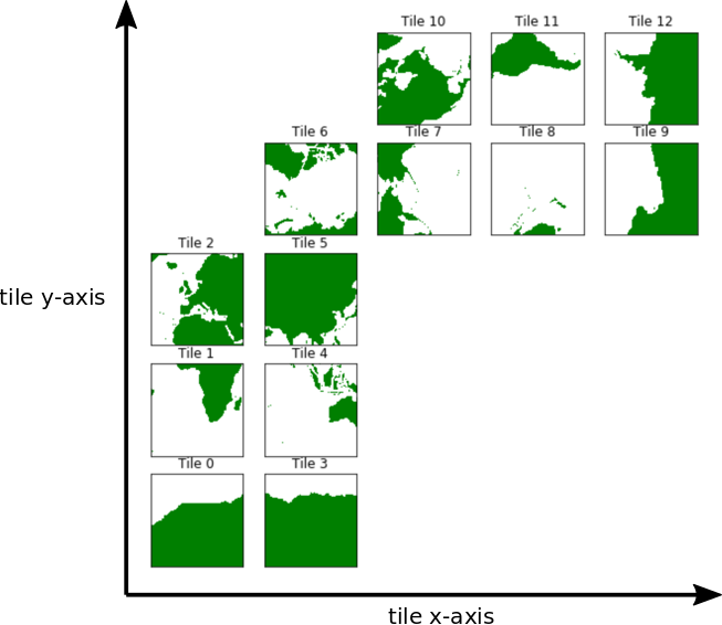
Tiles 7-12 are rotated 90 degrees counter-clockwise relative to tiles 0-5.
In this tutorial we demonstrate two methods for mapping scalar and vector fields from the llc90 model grid to “regular” latitude-longitude grids of arbitrary resolution.
Note: There are many methods on can use to map between the grids (e.g., nearest neighbor, bilinear interpolation, bin-averaging, etc.), each with its own advantages.)
In this tutorial we’ll use the ECCO grid file and monthly SSH and wind stress from the year 2000. The ecco_access package will handle download or retrieval of the necessary data, though you may need to install it. The ShortNames of the datasets are:
ECCO_L4_GEOMETRY_LLC0090GRID_V4R4
ECCO_L4_SSH_LLC0090GRID_MONTHLY_V4R4
ECCO_L4_STRESS_LLC0090GRID_MONTHLY_V4R4
How to interpolate scalar ECCO fields to a lat-lon grid
Scalar fields are the most straightforward fields to interpolate.
Preliminaries: Load fields
First, let’s load the all 13 tiles for sea surface height and the model grid parameters.
[1]:
import numpy as np
import sys
import xarray as xr
from os.path import join,expanduser
import matplotlib.pyplot as plt
%matplotlib inline
import glob
import warnings
warnings.filterwarnings('ignore')
from pprint import pprint
import importlib


import ecco_v4_py as ecco
import ecco_access as ea


# are you working in the AWS Cloud?
incloud_access = False

# indicate mode of access from PO.DAAC
# options are:
# 'download': direct download from internet to your local machine
# 'download_ifspace': like download, but only proceeds
#                     if your machine have sufficient storage
# 's3_open': access datasets in-cloud from an AWS instance
# 's3_open_fsspec': use jsons generated with fsspec and
#                   kerchunk libraries to speed up in-cloud access
# 's3_get': direct download from S3 in-cloud to an AWS instance
# 's3_get_ifspace': like s3_get, but only proceeds if your instance
#                   has sufficient storage
user_home_dir = expanduser('~')
download_dir = join(user_home_dir,'Downloads','ECCO_V4r4_PODAAC')
if incloud_access:
    access_mode = 's3_open_fsspec'
    download_root_dir = None
    jsons_root_dir = join(user_home_dir,'MZZ')
else:
    access_mode = 'download_ifspace'
    download_root_dir = download_dir
    jsons_root_dir = None
[4]:
## Access datasets needed for this tutorial

ShortNames_list = ["ECCO_L4_GEOMETRY_LLC0090GRID_V4R4",\
                   "ECCO_L4_SSH_LLC0090GRID_MONTHLY_V4R4",\
                   "ECCO_L4_STRESS_LLC0090GRID_MONTHLY_V4R4"]

ds_dict = ea.ecco_podaac_to_xrdataset(ShortNames_list,\
                                              StartDate='2000-01',EndDate='2000-12',\
                                              mode=access_mode,\
                                              download_root_dir=download_root_dir,\
                                              jsons_root_dir=jsons_root_dir,\
                                              max_avail_frac=0.5)
Size of files to be downloaded to instance is 0.14100000000000001 GB,
which is 0.1% of the 144.247 GB available storage.
Proceeding with file downloads via NASA Earthdata URLs
DL Progress: 100%|###########################| 1/1 [00:02<00:00,  2.48s/it]

=====================================
total downloaded: 8.57 Mb
avg download speed: 3.45 Mb/s
Time spent = 2.4872360229492188 seconds


DL Progress: 100%|#########################| 12/12 [00:04<00:00,  2.63it/s]

=====================================
total downloaded: 71.01 Mb
avg download speed: 15.55 Mb/s
Time spent = 4.5674521923065186 seconds


DL Progress: 100%|#########################| 12/12 [00:04<00:00,  2.73it/s]

=====================================
total downloaded: 71.55 Mb
avg download speed: 16.21 Mb/s
Time spent = 4.4131903648376465 seconds
[5]:
## Load the model grid
ecco_grid = ds_dict[ShortNames_list[0]].compute()
[6]:
## Load monthly SSH from 2000

ecco_vars = ds_dict[ShortNames_list[1]]

## Merge the ecco_grid with the ecco_vars to make the ecco_ds
ecco_ds = xr.merge((ecco_grid , ecco_vars)).compute()

pprint(ecco_ds.data_vars)
Data variables:
    CS        (tile, j, i) float32 421kB 0.06158 0.06675 ... -0.9854 -0.9984
    SN        (tile, j, i) float32 421kB -0.9981 -0.9978 ... -0.1705 -0.05718
    rA        (tile, j, i) float32 421kB 3.623e+08 3.633e+08 ... 3.611e+08
    dxG       (tile, j_g, i) float32 421kB 1.558e+04 1.559e+04 ... 2.314e+04
    dyG       (tile, j, i_g) float32 421kB 2.321e+04 2.327e+04 ... 1.558e+04
    Depth     (tile, j, i) float32 421kB 0.0 0.0 0.0 0.0 0.0 ... 0.0 0.0 0.0 0.0
    rAz       (tile, j_g, i_g) float32 421kB 1.799e+08 1.805e+08 ... 3.642e+08
    dxC       (tile, j, i_g) float32 421kB 1.558e+04 1.559e+04 ... 2.341e+04
    dyC       (tile, j_g, i) float32 421kB 1.156e+04 1.159e+04 ... 1.558e+04
    rAw       (tile, j, i_g) float32 421kB 3.617e+08 3.628e+08 ... 3.648e+08
    rAs       (tile, j_g, i) float32 421kB 1.802e+08 1.807e+08 ... 3.605e+08
    drC       (k_p1) float32 204B 5.0 10.0 10.0 10.0 ... 399.0 422.0 445.0 228.2
    drF       (k) float32 200B 10.0 10.0 10.0 10.0 ... 387.5 410.5 433.5 456.5
    PHrefC    (k) float32 200B 49.05 147.1 245.2 ... 5.357e+04 5.794e+04
    PHrefF    (k_p1) float32 204B 0.0 98.1 196.2 ... 5.57e+04 6.018e+04
    hFacC     (k, tile, j, i) float32 21MB 0.0 0.0 0.0 0.0 ... 0.0 0.0 0.0 0.0
    hFacW     (k, tile, j, i_g) float32 21MB 0.0 0.0 0.0 0.0 ... 0.0 0.0 0.0 0.0
    hFacS     (k, tile, j_g, i) float32 21MB 0.0 0.0 0.0 0.0 ... 0.0 0.0 0.0 0.0
    maskC     (k, tile, j, i) bool 5MB False False False ... False False False
    maskW     (k, tile, j, i_g) bool 5MB False False False ... False False False
    maskS     (k, tile, j_g, i) bool 5MB False False False ... False False False
    SSH       (time, tile, j, i) float32 5MB nan nan nan nan ... nan nan nan nan
    SSHIBC    (time, tile, j, i) float32 5MB nan nan nan nan ... nan nan nan nan
    SSHNOIBC  (time, tile, j, i) float32 5MB nan nan nan nan ... nan nan nan nan
    ETAN      (time, tile, j, i) float32 5MB nan nan nan nan ... nan nan nan nan
Plotting the dataset
Plotting the ECCOv4 fields was covered in an earlier tutorial. Before demonstrating interpolation, we will first plot one of our SSH fields. Take a closer look at the arguments of plot_proj_to_latlon_grid, dx=2 and dy=2.
[7]:
plt.figure(figsize=(12,6), dpi= 90)

tmp_plt = ecco_ds.SSH.isel(time=1)
tmp_plt = tmp_plt.where(ecco_ds.hFacC.isel(k=0) !=0)

ecco.plot_proj_to_latlon_grid(ecco_ds.XC, \
                              ecco_ds.YC, \
                              tmp_plt, \
                              plot_type = 'pcolormesh', \
                              dx=2,\
                              dy=2, \
                              projection_type = 'robin',\
                              less_output = True);

These dx and dy arguments tell the plotting function to interpolate the native grid tiles onto a lat-lon grid with spacing of dx degrees longitude and dy degrees latitude. If we reduced dx and dy the resulting map would have finer features: Compare with the map when dx=dy=0.25 degrees:
[8]:
plt.figure(figsize=(12,6), dpi= 90)

tmp_plt = ecco_ds.SSH.isel(time=1)
tmp_plt = tmp_plt.where(ecco_ds.hFacC.isel(k=0) !=0)

ecco.plot_proj_to_latlon_grid(ecco_ds.XC, \
                              ecco_ds.YC, \
                              tmp_plt, \
                              plot_type = 'pcolormesh', \
                              dx=0.25,\
                              dy=0.25, \
                              projection_type = 'robin',\
                              less_output = True);

Of course you can interpolate to arbitrarily high resolution lat-lon grids, the model resolution will ultimately determine the smallest resolvable features.
Under the hood of plot_proj_to_lat_longrid is a call to the very useful routine resample_to_latlon which is the now described in more detail
resample_to_latlon
resample_to_latlon takes a field with a cooresponding set of lat lon coordinates (the source grid) and interpolates to a new lat-lon target grid. The arrangement of coordinates in the source grid is arbitrary. One also provides the  of the new lat lon grid. The example shown above uses -90..90N and -180..180E by default. In addition, one specifies which interpolation scheme to use (mapping method) and the radius of influence, the radius around the target grid cells
within which to search for values from the source grid.
of the new lat lon grid. The example shown above uses -90..90N and -180..180E by default. In addition, one specifies which interpolation scheme to use (mapping method) and the radius of influence, the radius around the target grid cells
within which to search for values from the source grid.
[9]:
help(ecco.resample_to_latlon)
Help on function resample_to_latlon in module ecco_v4_py.resample_to_latlon:

resample_to_latlon(orig_lons, orig_lats, orig_field, new_grid_min_lat, new_grid_max_lat, new_grid_delta_lat, new_grid_min_lon, new_grid_max_lon, new_grid_delta_lon, radius_of_influence=120000, fill_value=None, mapping_method='bin_average')
    Take a field from a source grid and interpolate to a target grid.

    Parameters
    ----------
    orig_lons, orig_lats, orig_field : xarray DataArray or numpy array  :
        the lons, lats, and field from the source grid

        new_grid_min_lat, new_grid_max_lat : float
                latitude limits of new lat-lon grid

    new_grid_delta_lat : float
        latitudinal extent of new lat-lon grid cells in degrees (-90..90)

    new_grid_min_lon, new_grid_max_lon : float
                longitude limits of new lat-lon grid (-180..180)

    new_grid_delta_lon : float
         longitudinal extent of new lat-lon grid cells in degrees

    radius_of_influence : float, optional.  Default 120000 m
        the radius of the circle within which the input data is search for
        when mapping to the new grid

    fill_value : float, optional. Default None
                value to use in the new lat-lon grid if there are no valid values
                from the source grid

        mapping_method : string, optional. Default 'bin_average'
        denote the type of interpolation method to use.
        options include
            'nearest_neighbor' - Take the nearest value from the source grid
                                                 to the target grid
            'bin_average'      - Use the average value from the source grid
                                                                 to the target grid

    RETURNS:
    new_grid_lon_centers, new_grid_lat_centers : ndarrays
        2D arrays with the lon and lat values of the new grid cell centers

    new_grid_lon_edges, new_grid_lat_edges: ndarrays
        2D arrays with the lon and lat values of the new grid cell edges

    data_latlon_projection:
        the source field interpolated to the new grid
Demonstrations of resample_to_latlon
Global
First we will map to a global lat-lon grid at 1degree using nearest neighbor
[10]:
new_grid_delta_lat = 1
new_grid_delta_lon = 1

new_grid_min_lat = -90
new_grid_max_lat = 90

new_grid_min_lon = -180
new_grid_max_lon = 180

new_grid_lon_centers, new_grid_lat_centers,\
new_grid_lon_edges, new_grid_lat_edges,\
field_nearest_1deg =\
        ecco.resample_to_latlon(ecco_ds.XC, \
                                ecco_ds.YC, \
                                ecco_ds.SSH.isel(time=0),\
                                new_grid_min_lat, new_grid_max_lat, new_grid_delta_lat,\
                                new_grid_min_lon, new_grid_max_lon, new_grid_delta_lon,\
                                fill_value = np.NaN, \
                                mapping_method = 'nearest_neighbor',
                                radius_of_influence = 120000)
[11]:
# Dimensions of the new grid:
pprint(new_grid_lat_centers.shape)
pprint(new_grid_lon_centers.shape)
(180, 360)
(180, 360)
[12]:
pprint(new_grid_lon_centers)

# the second dimension of new_grid_lon has the center longitude of the new grid cells
pprint(new_grid_lon_centers[0,0:10])
array([[-179.5, -178.5, -177.5, ...,  177.5,  178.5,  179.5],
       [-179.5, -178.5, -177.5, ...,  177.5,  178.5,  179.5],
       [-179.5, -178.5, -177.5, ...,  177.5,  178.5,  179.5],
       ...,
       [-179.5, -178.5, -177.5, ...,  177.5,  178.5,  179.5],
       [-179.5, -178.5, -177.5, ...,  177.5,  178.5,  179.5],
       [-179.5, -178.5, -177.5, ...,  177.5,  178.5,  179.5]])
array([-179.5, -178.5, -177.5, -176.5, -175.5, -174.5, -173.5, -172.5,
       -171.5, -170.5])
[13]:
# The set of lat points
pprint(new_grid_lat_centers)

# or as a 1D vector
# the first dimension of new_grid_lat has the center latitude of the new grid cells
pprint(new_grid_lat_centers[0:10,0])
array([[-89.5, -89.5, -89.5, ..., -89.5, -89.5, -89.5],
       [-88.5, -88.5, -88.5, ..., -88.5, -88.5, -88.5],
       [-87.5, -87.5, -87.5, ..., -87.5, -87.5, -87.5],
       ...,
       [ 87.5,  87.5,  87.5, ...,  87.5,  87.5,  87.5],
       [ 88.5,  88.5,  88.5, ...,  88.5,  88.5,  88.5],
       [ 89.5,  89.5,  89.5, ...,  89.5,  89.5,  89.5]])
array([-89.5, -88.5, -87.5, -86.5, -85.5, -84.5, -83.5, -82.5, -81.5,
       -80.5])
[14]:
# plot the whole field
plt.figure(figsize=(12,6), dpi= 90)
plt.imshow(field_nearest_1deg,origin='lower')
[14]:
<matplotlib.image.AxesImage at 0x7f79c4173a50>

Regional
1 degree, nearest neighbor
First we’ll interpolate only to a subset of the N. Atlantic at 1 degree.
[15]:
new_grid_delta_lat = 1
new_grid_delta_lon = 1

new_grid_min_lat = 30
new_grid_max_lat = 82

new_grid_min_lon = -90
new_grid_max_lon = 10

new_grid_lon_centers, new_grid_lat_centers,\
new_grid_lon_edges, new_grid_lat_edges,\
field_nearest_1deg =\
        ecco.resample_to_latlon(ecco_ds.XC, \
                                ecco_ds.YC, \
                                ecco_ds.SSH.isel(time=0),\
                                new_grid_min_lat, new_grid_max_lat, new_grid_delta_lat,\
                                new_grid_min_lon, new_grid_max_lon, new_grid_delta_lon,\
                                fill_value = np.NaN, \
                                mapping_method = 'nearest_neighbor',
                                radius_of_influence = 120000)

# plot the whole field, this time land values are nans.
plt.figure(figsize=(8,6), dpi= 90)
plt.imshow(field_nearest_1deg,origin='lower',cmap='jet')
[15]:
<matplotlib.image.AxesImage at 0x7f79c56a0d90>

0.05 degree, nearest neighbor
Next we’ll interpolate the same domain at a much higher resolution, 0.05 degree:
[16]:
new_grid_delta_lat = 0.05
new_grid_delta_lon = 0.05

new_grid_min_lat = 30
new_grid_max_lat = 82

new_grid_min_lon = -90
new_grid_max_lon = 10


new_grid_lon_centers, new_grid_lat_centers,\
new_grid_lon_edges, new_grid_lat_edges,\
field_nearest_1deg =\
        ecco.resample_to_latlon(ecco_ds.XC, \
                                ecco_ds.YC, \
                                ecco_ds.SSH.isel(time=0),\
                                new_grid_min_lat, new_grid_max_lat, new_grid_delta_lat,\
                                new_grid_min_lon, new_grid_max_lon, new_grid_delta_lon,\
                                fill_value = np.NaN, \
                                mapping_method = 'nearest_neighbor',
                                radius_of_influence = 120000)

# plot the whole field, this time land values are nans.
plt.figure(figsize=(8,6), dpi= 90)
plt.imshow(field_nearest_1deg,origin='lower',cmap='jet');

The new grid is much finer than the llc90 grid. Because we are using the nearest neighbor method, you can make out the approximate size and location of the llc90 model grid cells (think about it: nearest neighbor).
0.05 degree, bin average
With bin averaging many values from the source grid are ‘binned’ together and then averaged to determine the value in the new grid. The numer of grid cells from the source grid depends on the source grid resolution and the radius of influence. If we were to choose a radius of influence of 120000 m (a little longer than 1 degree longitude at the equator) the interpolated lat-lon map would be smoother than if we were to choose a smaller radius. To demonstrate:
bin average with 120000 m radius
[17]:
new_grid_lon_centers, new_grid_lat_centers,\
new_grid_lon_edges, new_grid_lat_edges,\
field_nearest_1deg =\
        ecco.resample_to_latlon(ecco_ds.XC, \
                                ecco_ds.YC, \
                                ecco_ds.SSH.isel(time=0),\
                                new_grid_min_lat, new_grid_max_lat, new_grid_delta_lat,\
                                new_grid_min_lon, new_grid_max_lon, new_grid_delta_lon,\
                                fill_value = np.NaN, \
                                mapping_method = 'bin_average',
                                radius_of_influence = 120000)

# plot the whole field, this time land values are nans.
plt.figure(figsize=(8,6), dpi= 90)
plt.imshow(field_nearest_1deg,origin='lower',cmap='jet');

bin average with 40000m radius
[18]:
new_grid_lon_centers, new_grid_lat_centers,\
new_grid_lon_edges, new_grid_lat_edges,\
field_nearest_1deg =\
        ecco.resample_to_latlon(ecco_ds.XC, \
                                ecco_ds.YC, \
                                ecco_ds.SSH.isel(time=0),\
                                new_grid_min_lat, new_grid_max_lat, new_grid_delta_lat,\
                                new_grid_min_lon, new_grid_max_lon, new_grid_delta_lon,\
                                fill_value = np.NaN, \
                                mapping_method = 'bin_average',
                                radius_of_influence = 40000)

# plot the whole field, this time land values are nans.
plt.figure(figsize=(8,6), dpi= 90)
plt.imshow(field_nearest_1deg,origin='lower',cmap='jet');

You may wonder why there are missing (white) values in the resulting map. It’s because there are some lat-lon grid cells whose center is more than 40km away from the center of any grid cell on the source grid. There are ways to get around this problem by specifying spatially-varying radii of influence, but that will have to wait for another tutorial.
If you want to explore on your own, explore some of the low-level routines of the pyresample package: https://pyresample.readthedocs.io/en/latest/
Interpolating ECCO vectors fields to lat-lon grids
Vector fields require a few more steps to interpolate to the lat-lon grid. At least if what you want are the zonal and meridional vector components. Why? Because in the llc90 grid, vector fields like UVEL and VVEL are defined with positive in the +x and +y directions of the local coordinate system, respectively. A term like oceTAUX correponds to ocean wind stress in the +x direction and does not correspond to zonal wind stress. To calculate zonal wind stress we need to rotate the
vector from the llc90 x-y grid system to the lat-lon grid.
To demonstrate why rotation is necessary, consider the model field oceTAUX
[19]:
## Load vector fields

ecco_vars = ds_dict[ShortNames_list[2]]

## Merge the ecco_grid with the ecco_vars to make the ecco_ds
ecco_ds = xr.merge((ecco_grid , ecco_vars)).compute()

pprint(ecco_ds.data_vars)
Data variables:
    CS       (tile, j, i) float32 421kB 0.06158 0.06675 ... -0.9854 -0.9984
    SN       (tile, j, i) float32 421kB -0.9981 -0.9978 ... -0.1705 -0.05718
    rA       (tile, j, i) float32 421kB 3.623e+08 3.633e+08 ... 3.611e+08
    dxG      (tile, j_g, i) float32 421kB 1.558e+04 1.559e+04 ... 2.314e+04
    dyG      (tile, j, i_g) float32 421kB 2.321e+04 2.327e+04 ... 1.558e+04
    Depth    (tile, j, i) float32 421kB 0.0 0.0 0.0 0.0 0.0 ... 0.0 0.0 0.0 0.0
    rAz      (tile, j_g, i_g) float32 421kB 1.799e+08 1.805e+08 ... 3.642e+08
    dxC      (tile, j, i_g) float32 421kB 1.558e+04 1.559e+04 ... 2.341e+04
    dyC      (tile, j_g, i) float32 421kB 1.156e+04 1.159e+04 ... 1.558e+04
    rAw      (tile, j, i_g) float32 421kB 3.617e+08 3.628e+08 ... 3.648e+08
    rAs      (tile, j_g, i) float32 421kB 1.802e+08 1.807e+08 ... 3.605e+08
    drC      (k_p1) float32 204B 5.0 10.0 10.0 10.0 ... 399.0 422.0 445.0 228.2
    drF      (k) float32 200B 10.0 10.0 10.0 10.0 ... 387.5 410.5 433.5 456.5
    PHrefC   (k) float32 200B 49.05 147.1 245.2 ... 5.357e+04 5.794e+04
    PHrefF   (k_p1) float32 204B 0.0 98.1 196.2 ... 5.145e+04 5.57e+04 6.018e+04
    hFacC    (k, tile, j, i) float32 21MB 0.0 0.0 0.0 0.0 ... 0.0 0.0 0.0 0.0
    hFacW    (k, tile, j, i_g) float32 21MB 0.0 0.0 0.0 0.0 ... 0.0 0.0 0.0 0.0
    hFacS    (k, tile, j_g, i) float32 21MB 0.0 0.0 0.0 0.0 ... 0.0 0.0 0.0 0.0
    maskC    (k, tile, j, i) bool 5MB False False False ... False False False
    maskW    (k, tile, j, i_g) bool 5MB False False False ... False False False
    maskS    (k, tile, j_g, i) bool 5MB False False False ... False False False
    EXFtaux  (time, tile, j, i) float32 5MB nan nan nan nan ... nan nan nan nan
    EXFtauy  (time, tile, j, i) float32 5MB nan nan nan nan ... nan nan nan nan
    oceTAUX  (time, tile, j, i_g) float32 5MB nan nan nan nan ... nan nan nan
    oceTAUY  (time, tile, j_g, i) float32 5MB nan nan nan nan ... nan nan nan
[20]:
tmp = ecco_ds.oceTAUX.isel(time=0)
ecco.plot_tiles(tmp,cmap='coolwarm');

We can sees the expected positive zonal wind stress in tiles 0-5 because the x-y coordinates of tiles 0-5 happen to approximately line up with the meridians and parallels of the lat-lon grid. Importantly, for tiles 7-12 wind stress in the +x direction corresponds to mainly wind stress in the SOUTH direction. To see the zonal wind stress in tiles 7-12 one has to plot oceTAUY and recognize that for those tiles positive values correspond with wind stress in the tile’s +y direction, which is
approximately east-west. To wit,
[21]:
tmp = ecco_ds.oceTAUY.isel(time=0)
ecco.plot_tiles(tmp,cmap='coolwarm');

Great, but if you want zonal and meridional wind stress, we need to determine the zonal and meridional components of these vectors.
Vector rotation
For vector rotation we leverage the very useful XGCM package (https://xgcm.readthedocs.io/en/latest/).
Note: The XGCM documentation contains an MITgcm ECCOv4 Example Page: https://xgcm.readthedocs.io/en/latest/example_eccov4.html. In that example the dimension ‘tile’ is called ‘face’ and the fields were loaded from the binary output of the MITgcm, not the netCDF files that we produce for the official ECCOv4r4 product. Differences are largely cosmetic.)
We use XGCM to map the +x and +y vector components to the grid cell centers from the u and v grid points of the Arakawa C grid. The ecco-v4-py routine get_llc_grid creates the XGCM grid object using a DataSet object containing the following information about the model grid:
i,j,i_g,j_g,k,k_l,k_u,k_p1 .
Our ecco_ds DataSet does have these fields, they come from the grid file:
[22]:
# dimensions of the ecco_ds DataSet
ecco_ds.dims
[22]:
FrozenMappingWarningOnValuesAccess({'i': 90, 'i_g': 90, 'j': 90, 'j_g': 90, 'k': 50, 'k_u': 50, 'k_l': 50, 'k_p1': 51, 'tile': 13, 'nb': 4, 'nv': 2, 'time': 12})
[23]:
# Make the XGCM object
XGCM_grid = ecco.get_llc_grid(ecco_ds)

# look at the XGCM object.
XGCM_grid

# Depending on how much you want to geek out, you can learn about this fancy XGCM_grid object here:
# https://xgcm.readthedocs.io/en/latest/grid_topology.html
[23]:
<xgcm.Grid>
T Axis (not periodic, boundary=None):
  * center   time
Y Axis (not periodic, boundary=None):
  * center   j --> left
  * left     j_g --> center
X Axis (not periodic, boundary=None):
  * center   i --> left
  * left     i_g --> center
Z Axis (not periodic, boundary=None):
  * center   k --> left
  * right    k_u --> center
  * left     k_l --> center
  * outer    k_p1 --> center
Once we have the XGCM_grid object, we can use built-in routines of XGCM to interpolate the x and y components of a vector field to the cell centers.
[24]:
import xgcm
xfld = ecco_ds.oceTAUX.isel(time=0)
yfld = ecco_ds.oceTAUY.isel(time=0)

velc = XGCM_grid.interp_2d_vector({'X': xfld, 'Y': yfld},boundary='fill')
velc is a dictionary of the x and y vector components taken to the model grid cell centers. At this point they are not yet rotated!
[25]:
velc.keys()
[25]:
dict_keys(['X', 'Y'])
The magic comes here, with the use of the grid cosine ‘cs’ and grid sine ‘cs’ values from the ECCO grid file:
[26]:
# Compute the zonal and meridional vector components of oceTAUX and oceTAUY
oceTAU_E  = velc['X']*ecco_ds['CS'] - velc['Y']*ecco_ds['SN']
oceTAU_N  = velc['X']*ecco_ds['SN'] + velc['Y']*ecco_ds['CS']
Now we have the zonal and meridional components of the vectors, albeit still on the llc90 grid.
[27]:
ecco.plot_tiles(oceTAU_E,cmap='coolwarm');

So let’s resample oceTAU_E to a lat-lon grid (that’s why you’re here, right?) and plot
[28]:
new_grid_delta_lat = .5
new_grid_delta_lon = .5

new_grid_min_lat = -90
new_grid_max_lat = 90

new_grid_min_lon = -180
new_grid_max_lon = 180

new_grid_lon_centers, new_grid_lat_centers,\
new_grid_lon_edges, new_grid_lat_edges,\
oceTAU_E_latlon =\
        ecco.resample_to_latlon(ecco_ds.XC, \
                                ecco_ds.YC, \
                                oceTAU_E,\
                                new_grid_min_lat, new_grid_max_lat, new_grid_delta_lat,\
                                new_grid_min_lon, new_grid_max_lon, new_grid_delta_lon,\
                                fill_value = np.NaN, \
                                mapping_method = 'nearest_neighbor',
                                radius_of_influence = 120000)

# plot the resampled field
plt.figure(figsize=(12,8), dpi= 90);
plt.imshow(oceTAU_E_latlon,origin='lower',vmin=-.25,vmax=.25,cmap='coolwarm');
plt.title('ECCOv4 Jan 2000 Zonal Wind Stress (N/m^2)');
plt.colorbar(orientation='horizontal');

Or with extra fanciness:
[29]:
plt.figure(figsize=(12,6), dpi= 90)

ecco.plot_proj_to_latlon_grid(ecco_ds.XC, ecco_ds.YC, \
                              oceTAU_E, \
                              user_lon_0=180,\
                              projection_type='PlateCarree',\
                              plot_type = 'pcolormesh', \
                              dx=1,dy=1,show_colorbar=True,cmin=-.25, cmax=.25);

Compare vs “The Scatterometer Climatology of Ocean Winds (SCOW)”,
https://nanoos.ceoas.oregonstate.edu/scow/index.html
Risien, C.M., and D.B. Chelton, 2008: A Global Climatology of Surface Wind and Wind Stress Fields from Eight Years of QuikSCAT Scatterometer Data. J. Phys. Oceanogr., 38, 2379-2413.
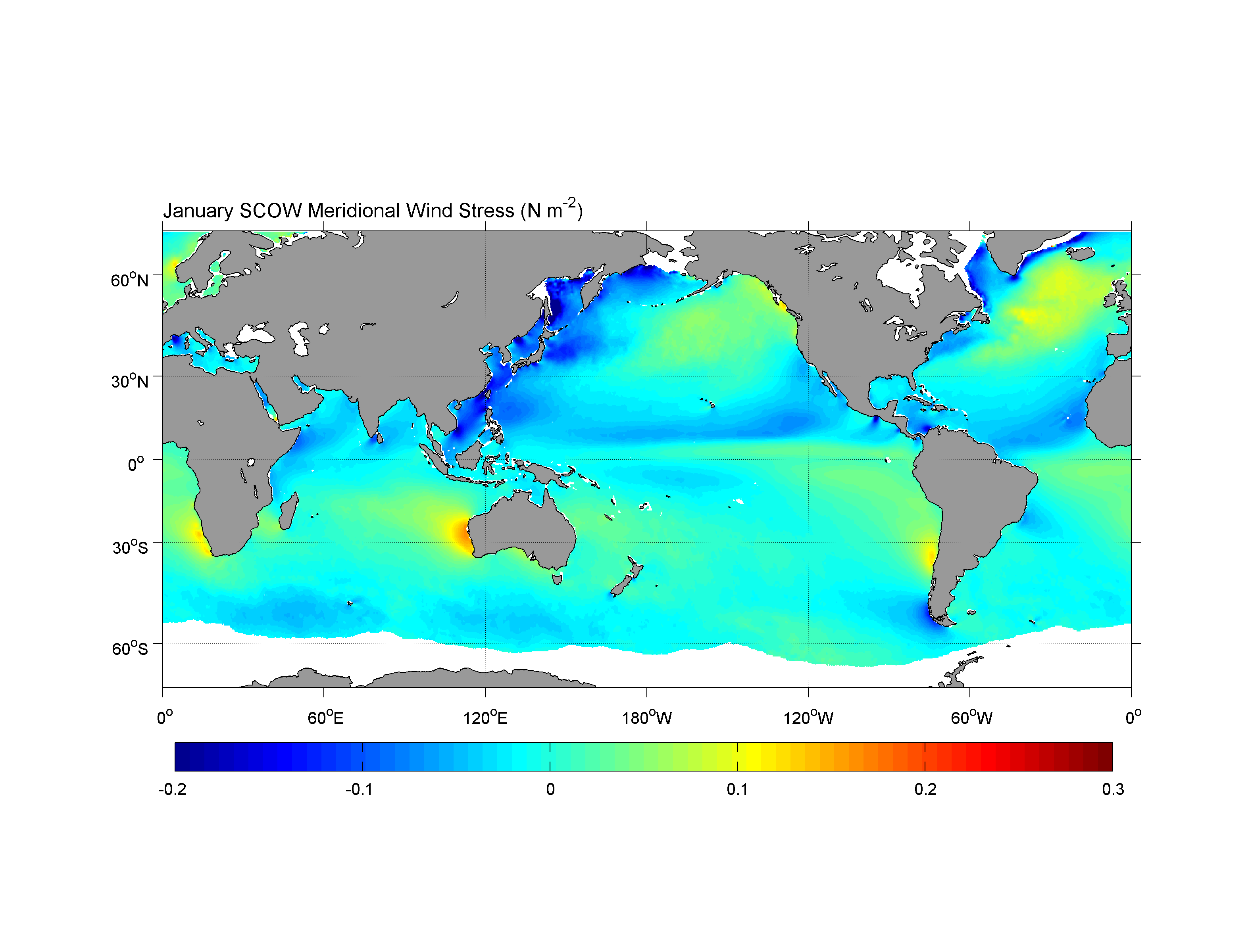
And of course we can’t forget about our meridional wind stress:
[30]:
plt.figure(figsize=(12,6), dpi= 90)
ecco.plot_proj_to_latlon_grid(ecco_ds.XC, ecco_ds.YC, \
                              oceTAU_N, \
                              user_lon_0=180,\
                              projection_type='PlateCarree',\
                              plot_type = 'pcolormesh', \
                              dx=1,dy=1,cmin=-.25, cmax=.25,show_colorbar=True);

Which we also compare against SCOW:
UEVNfromUXVY
The ecco-v4-py library includes a routine, UEVNfromUXVY which does the interpolation to the grid cell centers and the rotation in one call:
[31]:
xfld = ecco_ds.oceTAUX.isel(time=0)
yfld = ecco_ds.oceTAUY.isel(time=0)

# Compute the zonal and meridional vector components of oceTAUX and oceTAUY
oceTAU_E, oceTAU_N  = ecco.vector_calc.UEVNfromUXVY(xfld, yfld, ecco_ds)
Now plot to verify
[32]:
# interpolate to lat-lon
new_grid_lon_centers, new_grid_lat_centers,\
new_grid_lon_edges, new_grid_lat_edges,\
oceTAU_E_latlon =\
        ecco.resample_to_latlon(ecco_ds.XC, \
                                ecco_ds.YC, \
                                oceTAU_E,\
                                new_grid_min_lat, new_grid_max_lat, new_grid_delta_lat,\
                                new_grid_min_lon, new_grid_max_lon, new_grid_delta_lon,\
                                fill_value = np.NaN, \
                                mapping_method = 'nearest_neighbor',
                                radius_of_influence = 120000)

# plot the whole field, this time land values are nans.
plt.figure(figsize=(12,8), dpi= 90);
plt.imshow(oceTAU_E_latlon,origin='lower',vmin=-.25,vmax=.25,cmap='coolwarm');
plt.title('ECCOv4 Jan 2000 Zonal Wind Stress (N/m^2)');
plt.colorbar(orientation='horizontal');

Saving interpolated fields to netCDF
For this demonstration we will rotate the 12 monthly-mean records of oceTAUX and oceTAUY to their zonal and meridional components, interpolate to a lat-lon grids, and then save the output as netCDF format.
[33]:
pprint(ecco_ds.oceTAUX.time)
<xarray.DataArray 'time' (time: 12)> Size: 96B
array(['2000-01-16T12:00:00.000000000', '2000-02-15T12:00:00.000000000',
       '2000-03-16T12:00:00.000000000', '2000-04-16T00:00:00.000000000',
       '2000-05-16T12:00:00.000000000', '2000-06-16T00:00:00.000000000',
       '2000-07-16T12:00:00.000000000', '2000-08-16T12:00:00.000000000',
       '2000-09-16T00:00:00.000000000', '2000-10-16T12:00:00.000000000',
       '2000-11-16T00:00:00.000000000', '2000-12-16T12:00:00.000000000'],
      dtype='datetime64[ns]')
Coordinates:
  * time     (time) datetime64[ns] 96B 2000-01-16T12:00:00 ... 2000-12-16T12:...
Attributes:
    long_name:              center time of averaging period
    axis:                   T
    bounds:                 time_bnds
    coverage_content_type:  coordinate
    standard_name:          time
We will loop through each month, use UEVNfromUXVY to determine the zonal and meridional components of the ocean wind stress vectors, and then interpolate to a 0.5 degree lat-lon grid.
[34]:
oceTAUE = np.zeros((12,360,720))
oceTAUN = np.zeros((12,360,720))

new_grid_delta_lat = .5
new_grid_delta_lon = .5

new_grid_min_lat = -90
new_grid_max_lat = 90

new_grid_min_lon = -180
new_grid_max_lon = 180


for m in range(12):
    cur_oceTAUX = ecco_ds.oceTAUX.isel(time=m)
    cur_oceTAUY = ecco_ds.oceTAUY.isel(time=m)

    # Compute the zonal and meridional vector components of oceTAUX and oceTAUY
    tmp_e, tmp_n  = ecco.vector_calc.UEVNfromUXVY(cur_oceTAUX, cur_oceTAUY, ecco_ds)

    # zonal component
    new_grid_lon_centers, new_grid_lat_centers,\
    new_grid_lon_edges, new_grid_lat_edges,\
    tmp_e_latlon =\
        ecco.resample_to_latlon(ecco_ds.XC, \
                                ecco_ds.YC, \
                                tmp_e,\
                                new_grid_min_lat, new_grid_max_lat, new_grid_delta_lat,\
                                new_grid_min_lon, new_grid_max_lon, new_grid_delta_lon,\
                                fill_value = np.NaN, \
                                mapping_method = 'nearest_neighbor',
                                radius_of_influence = 120000)

    # meridional component
    new_grid_lon_centers, new_grid_lat_centers,\
    new_grid_lon_edges, new_grid_lat_edges,\
    tmp_n_latlon =\
        ecco.resample_to_latlon(ecco_ds.XC, \
                                ecco_ds.YC, \
                                tmp_n,\
                                new_grid_min_lat, new_grid_max_lat, new_grid_delta_lat,\
                                new_grid_min_lon, new_grid_max_lon, new_grid_delta_lon,\
                                fill_value = np.NaN, \
                                mapping_method = 'nearest_neighbor',
                                radius_of_influence = 120000)

    oceTAUE[m,:] = tmp_e_latlon
    oceTAUN[m,:] = tmp_n_latlon
[35]:
# make the new data array structures for the zonal and meridional wind stress fields
oceTAUE_DA = xr.DataArray(oceTAUE,  name = 'oceTAUE',
                      dims = ['time','latitude','longitude'],
                      coords = {'latitude': new_grid_lat_centers[:,0],
                                'longitude': new_grid_lon_centers[0,:],
                                'time': ecco_ds.time})

# make the new data array structures for the zonal and meridional wind stress fields
oceTAUN_DA = xr.DataArray(oceTAUN,  name = 'oceTAUN',
                      dims = ['time','latitude','longitude'],
                      coords = {'latitude': new_grid_lat_centers[:,0],
                                'longitude': new_grid_lon_centers[0,:],
                                'time': ecco_ds.time})
Plot the zonal and meridional wind stresses in these new DataArray objects:
[36]:
oceTAUE_DA.dims
[36]:
('time', 'latitude', 'longitude')
[37]:
oceTAUE_DA.isel(time=0).plot(cmap='RdYlBu_r')
[37]:
<matplotlib.collections.QuadMesh at 0x7f79a7446a10>

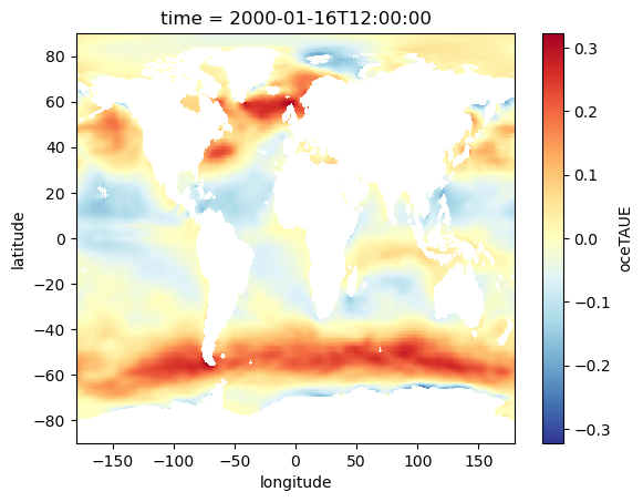
[38]:
oceTAUN_DA.isel(time=0).plot(cmap='RdYlBu_r')
[38]:
<matplotlib.collections.QuadMesh at 0x7f79a73695d0>
Saving is easy with xarray
[39]:
# meridional component
output_path = join(user_home_dir,'Downloads','oceTAUN_latlon_2000.nc')
oceTAUN_DA.to_netcdf(output_path)

# zonal component
output_path = join(user_home_dir,'Downloads','oceTAUE_latlon_2000.nc')
oceTAUE_DA.to_netcdf(output_path)
… done!