Accessing and Subsetting Variables

Objectives

Introduce methods for accessing and subsetting the variables stored in ECCO Datasets and DataArrays.

Introduction

There are two methods for accessing variables stored in DataArray and Dataset objects, the “dot” method and the “dictionary” method. The syntax of these methods is as follows:

1. The “dot” method: e.g. ,X.Y

2. The “dictionary” method: e.g., Y['Y']

Both methods work identically to access Dimensions, Coordinates, and Data variables. Accessing Attribute variables requires a slightly different approach as we will see.

For this tutorial make sure that you have the 2010 monthly granules of the SSH and OBP datasets downloaded, with ShortNames:

• ECCO_L4_SSH_LLC0090GRID_MONTHLY_V4R4

• ECCO_L4_OBP_LLC0090GRID_MONTHLY_V4R4

You will also need the grid file downloaded if you don’t have it already.

Accessing fields inside Dataset and DataArray objects

First create a Dataset:

import numpy as np
import xarray as xr
import sys
import matplotlib.pyplot as plt
%matplotlib inline
import json
import glob

import warnings
warnings.filterwarnings('ignore')

## Import the ecco_v4_py library into Python
## =========================================
##    If ecco_v4_py is not installed in your local Python library,
##    tell Python where to find it.  The example below adds
##    ecco_v4_py to the user's path if it is stored in the folder
##    ECCOv4-py under the user's home directory

from os.path import join,expanduser
user_home_dir = expanduser('~')

sys.path.append(join(user_home_dir,'ECCOv4-py'))

import ecco_v4_py as ecco

## Set top-level file directory for the ECCO NetCDF files
## =================================================================

## currently set to ~/Downloads/ECCO_V4r4_PODAAC,
## the default if ecco_podaac_download was used to download dataset granules
ECCO_dir = join(user_home_dir,'Downloads','ECCO_V4r4_PODAAC')

## Load the model grid
ecco_grid = xr.open_dataset(glob.glob(join(ECCO_dir,'*GEOMETRY*','*.nc'))[0])

## Load one year of SSH and OBP
ds_SSH = xr.open_mfdataset(join(ECCO_dir,'*SSH*MONTHLY*','*_2010-*.nc'))
ds_OBP = xr.open_mfdataset(join(ECCO_dir,'*OBP*MONTHLY*','*_2010-*.nc'))


## Merge the grid and variable datasets to make the ecco_ds
ecco_ds = xr.merge((ecco_grid,ds_SSH,ds_OBP))

ecco_ds.data_vars

Data variables:
    CS        (tile, j, i) float32 ...
    SN        (tile, j, i) float32 ...
    rA        (tile, j, i) float32 ...
    dxG       (tile, j_g, i) float32 ...
    dyG       (tile, j, i_g) float32 ...
    Depth     (tile, j, i) float32 ...
    rAz       (tile, j_g, i_g) float32 ...
    dxC       (tile, j, i_g) float32 ...
    dyC       (tile, j_g, i) float32 ...
    rAw       (tile, j, i_g) float32 ...
    rAs       (tile, j_g, i) float32 ...
    drC       (k_p1) float32 ...
    drF       (k) float32 ...
    PHrefC    (k) float32 ...
    PHrefF    (k_p1) float32 ...
    hFacC     (k, tile, j, i) float32 ...
    hFacW     (k, tile, j, i_g) float32 ...
    hFacS     (k, tile, j_g, i) float32 ...
    maskC     (k, tile, j, i) bool ...
    maskW     (k, tile, j, i_g) bool ...
    maskS     (k, tile, j_g, i) bool ...
    SSH       (time, tile, j, i) float32 dask.array<chunksize=(1, 13, 90, 90), meta=np.ndarray>
    SSHIBC    (time, tile, j, i) float32 dask.array<chunksize=(1, 13, 90, 90), meta=np.ndarray>
    SSHNOIBC  (time, tile, j, i) float32 dask.array<chunksize=(1, 13, 90, 90), meta=np.ndarray>
    ETAN      (time, tile, j, i) float32 dask.array<chunksize=(1, 13, 90, 90), meta=np.ndarray>
    OBP       (time, tile, j, i) float32 dask.array<chunksize=(1, 13, 90, 90), meta=np.ndarray>
    OBPGMAP   (time, tile, j, i) float32 dask.array<chunksize=(1, 13, 90, 90), meta=np.ndarray>
    PHIBOT    (time, tile, j, i) float32 dask.array<chunksize=(1, 13, 90, 90), meta=np.ndarray>

ecco_ds.coords

Coordinates:
  * i          (i) int32 0 1 2 3 4 5 6 7 8 9 ... 80 81 82 83 84 85 86 87 88 89
  * i_g        (i_g) int32 0 1 2 3 4 5 6 7 8 9 ... 80 81 82 83 84 85 86 87 88 89
  * j          (j) int32 0 1 2 3 4 5 6 7 8 9 ... 80 81 82 83 84 85 86 87 88 89
  * j_g        (j_g) int32 0 1 2 3 4 5 6 7 8 9 ... 80 81 82 83 84 85 86 87 88 89
  * k          (k) int32 0 1 2 3 4 5 6 7 8 9 ... 40 41 42 43 44 45 46 47 48 49
  * k_u        (k_u) int32 0 1 2 3 4 5 6 7 8 9 ... 40 41 42 43 44 45 46 47 48 49
  * k_l        (k_l) int32 0 1 2 3 4 5 6 7 8 9 ... 40 41 42 43 44 45 46 47 48 49
  * k_p1       (k_p1) int32 0 1 2 3 4 5 6 7 8 9 ... 42 43 44 45 46 47 48 49 50
  * tile       (tile) int32 0 1 2 3 4 5 6 7 8 9 10 11 12
    XC         (tile, j, i) float32 dask.array<chunksize=(13, 90, 90), meta=np.ndarray>
    YC         (tile, j, i) float32 dask.array<chunksize=(13, 90, 90), meta=np.ndarray>
    XG         (tile, j_g, i_g) float32 dask.array<chunksize=(13, 90, 90), meta=np.ndarray>
    YG         (tile, j_g, i_g) float32 dask.array<chunksize=(13, 90, 90), meta=np.ndarray>
    Z          (k) float32 ...
    Zp1        (k_p1) float32 ...
    Zu         (k_u) float32 ...
    Zl         (k_l) float32 ...
    XC_bnds    (tile, j, i, nb) float32 dask.array<chunksize=(13, 90, 90, 4), meta=np.ndarray>
    YC_bnds    (tile, j, i, nb) float32 dask.array<chunksize=(13, 90, 90, 4), meta=np.ndarray>
    Z_bnds     (k, nv) float32 ...
  * time       (time) datetime64[ns] 2010-01-16T12:00:00 ... 2010-12-16T12:00:00
    time_bnds  (time, nv) datetime64[ns] dask.array<chunksize=(1, 2), meta=np.ndarray>

Accessing Data Variables

Now we’ll use the two methods to access the SSH DataArray,

## The Dot Method
ssh_A = ecco_ds.SSH

## The Dictionary Method
ssh_B = ecco_ds['SSH']

print (type(ssh_A))
print (type(ssh_B))

<class 'xarray.core.dataarray.DataArray'>
<class 'xarray.core.dataarray.DataArray'>

We access the numpy arrays stored in these DataArrays with the “dot” method on values.

ssh_arr = ssh_A.values
print (type(ssh_arr))

<class 'numpy.ndarray'>

The numpy array storing the data

The shape of the numpy array can be found by invoking its .shape

ssh_arr.shape

(12, 13, 90, 90)

The order of these four dimensions is consistent with their ordering in the original DataArray, ~~~ time, tile, j, i ~~~

ssh_A.dims

('time', 'tile', 'j', 'i')

ssh_A and ssh_B are new variables but they are not copies of the original SSH DataArray object, they both point to the original numpy array.

We can confirm that ssh_A and ssh_B both refer to the same array in memory using the Python allclose command (and ignoring nans)

print(np.allclose(ssh_A, ssh_B, equal_nan=True))

True

Accessing the numpy array

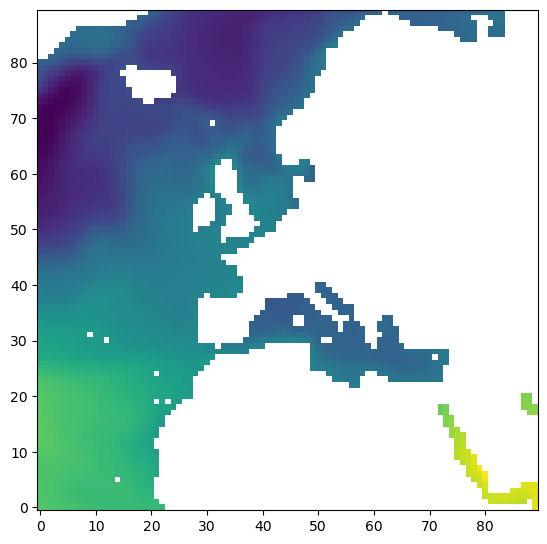
We have ssh_arr, a 4D numpy array (ndarray). Let’s take out a single 2D slice of it, the first time record, and the second tile:

fig=plt.figure(figsize=(8, 6.5))

# plot SSH for time =0, tile = 2 by using ``imshow`` on the ``numpy array``
plt.imshow(ssh_arr[0,2,:,:], origin='lower')

<matplotlib.image.AxesImage at 0x1ce9b963760>

We could accessing the array using the “dot” method on ecco_ds to first get SSH and then use the “dot” method to access the numpy array through values:

fig=plt.figure(figsize=(8, 6.5))
plt.imshow(ecco_ds.SSH.values[0,2,:,:], origin='lower')

<matplotlib.image.AxesImage at 0x1ce9d886a30>

Or could use the “dictionary” method on ecco_ds to get SSH then the “dot” method to access the numpy array through values:

fig=plt.figure(figsize=(8, 6.5))
plt.imshow(ecco_ds['SSH'].values[0,2,:,:], origin='lower')

<matplotlib.image.AxesImage at 0x1ce99245f70>

These are equivalent methods.

Accessing Coordinates

Accessing Coordinates is exactly the same as accessing Data variables. Use the “dot” or “dictionary” methods

xc = ecco_ds['XC']
time = ecco_ds['time']

print(type(xc))
print(type(time))

<class 'xarray.core.dataarray.DataArray'>
<class 'xarray.core.dataarray.DataArray'>

As xc is a DataArray, we can access the values in its numpy array through .values

xc.values

array([[[-111.60647 , -111.303   , -110.94285 , ...,   64.791115,
           64.80521 ,   64.81917 ],
        [-104.8196  , -103.928444, -102.87706 , ...,   64.36745 ,
           64.41012 ,   64.4524  ],
        [ -98.198784,  -96.788055,  -95.14185 , ...,   63.936497,
           64.008224,   64.0793  ],
        ...,
        [ -37.5     ,  -36.5     ,  -35.5     , ...,   49.5     ,
           50.5     ,   51.5     ],
        [ -37.5     ,  -36.5     ,  -35.5     , ...,   49.5     ,
           50.5     ,   51.5     ],
        [ -37.5     ,  -36.5     ,  -35.5     , ...,   49.5     ,
           50.5     ,   51.5     ]],

       [[ -37.5     ,  -36.5     ,  -35.5     , ...,   49.5     ,
           50.5     ,   51.5     ],
        [ -37.5     ,  -36.5     ,  -35.5     , ...,   49.5     ,
           50.5     ,   51.5     ],
        [ -37.5     ,  -36.5     ,  -35.5     , ...,   49.5     ,
           50.5     ,   51.5     ],
        ...,
        [ -37.5     ,  -36.5     ,  -35.5     , ...,   49.5     ,
           50.5     ,   51.5     ],
        [ -37.5     ,  -36.5     ,  -35.5     , ...,   49.5     ,
           50.5     ,   51.5     ],
        [ -37.5     ,  -36.5     ,  -35.5     , ...,   49.5     ,
           50.5     ,   51.5     ]],

       [[ -37.5     ,  -36.5     ,  -35.5     , ...,   49.5     ,
           50.5     ,   51.5     ],
        [ -37.5     ,  -36.5     ,  -35.5     , ...,   49.5     ,
           50.5     ,   51.5     ],
        [ -37.5     ,  -36.5     ,  -35.5     , ...,   49.5     ,
           50.5     ,   51.5     ],
        ...,
        [ -37.730072,  -37.17829 ,  -36.597565, ...,   50.597565,
           51.17829 ,   51.730072],
        [ -37.771988,  -37.291943,  -36.764027, ...,   50.764027,
           51.291943,   51.771988],
        [ -37.837925,  -37.44421 ,  -36.968143, ...,   50.968143,
           51.44421 ,   51.837925]],

       ...,

       [[-127.83792 , -127.77199 , -127.73007 , ..., -127.5     ,
         -127.5     , -127.5     ],
        [-127.44421 , -127.29195 , -127.17829 , ..., -126.5     ,
         -126.5     , -126.5     ],
        [-126.96814 , -126.76402 , -126.597565, ..., -125.5     ,
         -125.5     , -125.5     ],
        ...,
        [ -39.031857,  -39.235973,  -39.402435, ...,  -40.5     ,
          -40.5     ,  -40.5     ],
        [ -38.55579 ,  -38.708057,  -38.82171 , ...,  -39.5     ,
          -39.5     ,  -39.5     ],
        [ -38.162075,  -38.228012,  -38.269928, ...,  -38.5     ,
          -38.5     ,  -38.5     ]],

       [[-127.5     , -127.5     , -127.5     , ..., -127.5     ,
         -127.5     , -127.5     ],
        [-126.5     , -126.5     , -126.5     , ..., -126.5     ,
         -126.5     , -126.5     ],
        [-125.5     , -125.5     , -125.5     , ..., -125.5     ,
         -125.5     , -125.5     ],
        ...,
        [ -40.5     ,  -40.5     ,  -40.5     , ...,  -40.5     ,
          -40.5     ,  -40.5     ],
        [ -39.5     ,  -39.5     ,  -39.5     , ...,  -39.5     ,
          -39.5     ,  -39.5     ],
        [ -38.5     ,  -38.5     ,  -38.5     , ...,  -38.5     ,
          -38.5     ,  -38.5     ]],

       [[-127.5     , -127.5     , -127.5     , ..., -115.850204,
         -115.50567 , -115.166985],
        [-126.5     , -126.5     , -126.5     , ..., -115.78025 ,
         -115.464066, -115.153244],
        [-125.5     , -125.5     , -125.5     , ..., -115.71079 ,
         -115.42275 , -115.139595],
        ...,
        [ -40.5     ,  -40.5     ,  -40.5     , ..., -101.42989 ,
         -106.83081 , -112.28605 ],
        [ -39.5     ,  -39.5     ,  -39.5     , ..., -100.48844 ,
         -106.24874 , -112.090065],
        [ -38.5     ,  -38.5     ,  -38.5     , ...,  -99.42048 ,
         -105.58465 , -111.86579 ]]], dtype=float32)

The shape of the xc is 13 x 90 x 90. Unlike SSH there is no time dimension.

xc.values.shape

(13, 90, 90)

Accessing Attributes

To access Attribute fields you you can use the dot method directly on the Dataset or DataArray or the dictionary method on the attrs field.

To demonstrate: we access the units attribute on OBP using both methods

ecco_ds.OBP.units

'm'

ecco_ds.OBP.attrs['units']

'm'

Subsetting variables using the[], sel, isel, and where syntaxes

So far, a considerable amount of attention has been placed on the Coordinates of Dataset and DataArray objects. Why? Labeled coordinates are certainly not necessary for calculations on the basic numerical arrays that store the ECCO state estimate fields. The reason so much attention has been placed on coordinates is because the xarray offers several very useful methods for selecting (or indexing) subsets of data.

For more details of these indexing methods, please see the excellent xarray documentation: http://xarray.pydata.org/en/stable/indexing.html

Subsetting numpy arrays using the [ ] syntax

Subsetting numpy arrays is simple with the standard Python [ ] syntax.

To demonstrate, we’ll pull out the numpy array of SSH and then select the first time record and second tile

Note: numpy array indexing starts with 0*

ssh_arr = ecco_ds.SSH.values
type(ssh_arr)
ssh_arr.shape

(12, 13, 90, 90)

We know the order of the dimensions of SSH is [time, tile, j, i], so :

ssh_time_0_tile_2 = ssh_arr[0,2,:,:]

ssh_time_0_tile_2 is also a numpy array, but now it is a 2D array:

ssh_time_0_tile_2.shape

(90, 90)

Note that when subsetting only one index along a given dimension, numpy collapses (removes) that dimension by default. If you want to retain these “singleton” dimensions (sometimes useful for broadcasting the array) you can add brackets around the single index:

ssh_time_0_tile_2_3d = ssh_arr[[0],2,:,:]
ssh_time_0_tile_2_3d.shape

(1, 90, 90)

If you are subsetting a single index along multiple dimensions simultaneously, you may need to add extra brackets to retain the earlier dimensions:

ssh_time_0_tile_2_4d = ssh_arr[[[0]],[2],:,:]
ssh_time_0_tile_2_4d.shape

(1, 1, 90, 90)

We know that the time coordinate on ecco_ds has one dimension, time, so we can use the [] syntax to find the first element of that array as well:

print(ecco_ds.time.dims)

# the first time record is
print(ecco_ds.time.values[0])

('time',)
2010-01-16T12:00:00.000000000

which confirms that the first time record corresponds with Jan 2010

Now that we have a 2D array in ssh_time_0_tile_2, let’s plot it

fig=plt.figure(figsize=(8, 6.5))
plt.imshow(ssh_time_0_tile_2, origin='lower',cmap='jet')
plt.colorbar()
plt.title('<SSH> of Tile 2 for Jan 2010 [m]');
plt.xlabel('x-index');
plt.ylabel('y-index');

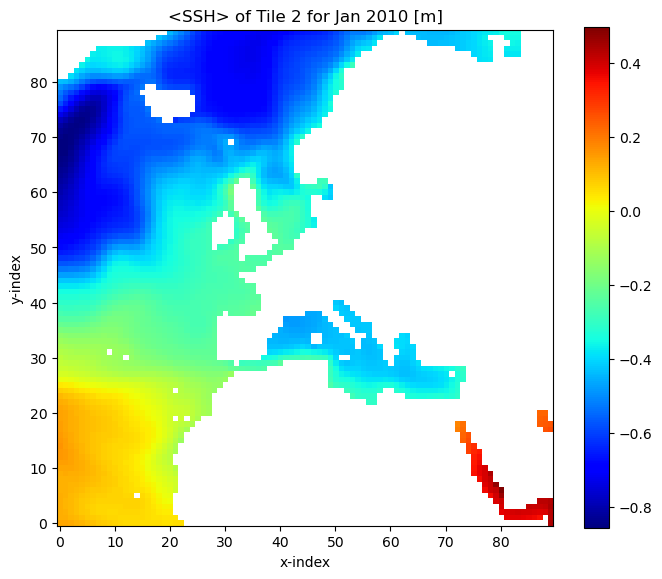
By eye we see large negative values around x=0, y=70 (i=0, j=70). Let’s confirm:

# remember the order of the array is [tile, j, i]
ssh_time_0_tile_2[70,0]

-0.84380484

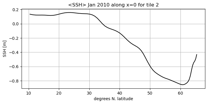
Let’s plot SSH in this tile from y=0 to y=89 along x=0 (from the subtropical gyre into the subpolar gyre)

fig=plt.figure(figsize=(8, 3.5))

plt.plot(ssh_time_0_tile_2[:,0])
plt.title('<SSH> Jan2010 along x=0 for tile 2')
plt.ylabel('SSH [m]');plt.xlabel('x index (no dimension)');
plt.grid()

We see that the curve stops at y=80 (rather than y=90), because from around y=80 on we are on Greenland and the array has nan values.

A more interesting plot might be to have the model latitude on the x axis instead of x-index:

fig=plt.figure(figsize=(8, 3.5))

yc_tile_2 = ecco_ds.YC.values[2,:,:]

plt.plot(yc_tile_2[:,0],ssh_time_0_tile_2[:,0], color='k')
plt.title('<SSH> Jan 2010 along x=0 for tile 2')
plt.ylabel('SSH [m]');plt.xlabel('degrees N. latitude');
plt.grid()

We can always use [ ] method to subset our numpy arrays. It is a simple, direct method for accessing our fields.

Subsetting DataArrays using the [ ] syntax

An interesting and useful alternative to subsetting numpy arrays with the [ ] method is to subset DataArray instead:

ssh_time_0_tile_2_DA = ecco_ds.SSH[0,2,:,:]
ssh_time_0_tile_2_DA

<xarray.DataArray 'SSH' (j: 90, i: 90)>
dask.array<getitem, shape=(90, 90), dtype=float32, chunksize=(90, 90), chunktype=numpy.ndarray>
Coordinates:
  * i        (i) int32 0 1 2 3 4 5 6 7 8 9 10 ... 80 81 82 83 84 85 86 87 88 89
  * j        (j) int32 0 1 2 3 4 5 6 7 8 9 10 ... 80 81 82 83 84 85 86 87 88 89
    tile     int32 2
    XC       (j, i) float32 dask.array<chunksize=(90, 90), meta=np.ndarray>
    YC       (j, i) float32 dask.array<chunksize=(90, 90), meta=np.ndarray>
    time     datetime64[ns] 2010-01-16T12:00:00
Attributes:
    long_name:              Dynamic sea surface height anomaly
    units:                  m
    coverage_content_type:  modelResult
    standard_name:          sea_surface_height_above_geoid
    comment:                Dynamic sea surface height anomaly above the geoi...
    valid_min:              -1.8805772066116333
    valid_max:              1.4207719564437866

The resulting DataArray is a subset of the original DataArray. The subset has two fewer dimensions (tile and time have been eliminated). The horizontal dimensions j and i are unchanged.

Even though the tile and time dimensions have been eliminated, the dimensional and non-dimensional coordinates associated with time and tile remain. In fact, these coordinates tell us when in time and which tile our subset comes from:

Coordinates:
  * j        (j) int64 0 1 2 3 4 5 6 7 8 9 10 ... 80 81 82 83 84 85 86 87 88 89
  * i        (i) int64 0 1 2 3 4 5 6 7 8 9 10 ... 80 81 82 83 84 85 86 87 88 89
    tile     int64 2
    XC       (j, i) float32 -37.5 -36.5 -35.5 ... 50.968143 51.44421 51.837925
    YC       (j, i) float32 10.458642 10.458642 10.458642 ... 67.53387 67.47211
    Depth    (j, i) float32 4658.681 4820.5703 5014.177 ... 0.0 0.0 0.0
    rA       (j, i) float32 11896091000.0 11896091000.0 ... 212633870.0
    iter     int32 158532
    time     datetime64[ns] 2010-01-16T12:00:00

Notice that the tile coordinate is 2 and the time coordinate is Jan 16, 2010, the middle of Jan.

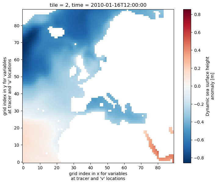
As a DataArray we can take full advantage of the built-in plotting functionality of xarray. This functionality, which we’ve seen a few times, automatically labels the figure (although sometimes the labels can be a little odd).

fig=plt.figure(figsize=(8, 6.5))
ssh_time_0_tile_2_DA.plot()

<matplotlib.collections.QuadMesh at 0x1ce972f1610>

Subsetting DataArrays using the .sel( ) syntax

Another useful method for subsetting DataArrays is the .sel( ) syntax. The .sel( ) syntax takes advantage of the fact that coordinates are labels. We select subsets of the DataArray by providing a subset of coordinate labels.

Let’s select tile 2 and time 2010-01-16:

ssh_time_0_tile_2_sel = ecco_ds.SSH.sel(time='2010-01-16', tile=2)
ssh_time_0_tile_2_sel

<xarray.DataArray 'SSH' (time: 1, j: 90, i: 90)>
dask.array<getitem, shape=(1, 90, 90), dtype=float32, chunksize=(1, 90, 90), chunktype=numpy.ndarray>
Coordinates:
  * i        (i) int32 0 1 2 3 4 5 6 7 8 9 10 ... 80 81 82 83 84 85 86 87 88 89
  * j        (j) int32 0 1 2 3 4 5 6 7 8 9 10 ... 80 81 82 83 84 85 86 87 88 89
    tile     int32 2
    XC       (j, i) float32 dask.array<chunksize=(90, 90), meta=np.ndarray>
    YC       (j, i) float32 dask.array<chunksize=(90, 90), meta=np.ndarray>
  * time     (time) datetime64[ns] 2010-01-16T12:00:00
Attributes:
    long_name:              Dynamic sea surface height anomaly
    units:                  m
    coverage_content_type:  modelResult
    standard_name:          sea_surface_height_above_geoid
    comment:                Dynamic sea surface height anomaly above the geoi...
    valid_min:              -1.8805772066116333
    valid_max:              1.4207719564437866

The only difference here is that the resulting array has ‘time’ as a singleton dimension (dimension of length 1). I don’t know why. Just use the squeeze command to squeeze it out.

ssh_time_0_tile_2_sel = ssh_time_0_tile_2_sel.squeeze()
ssh_time_0_tile_2_sel

<xarray.DataArray 'SSH' (j: 90, i: 90)>
dask.array<getitem, shape=(90, 90), dtype=float32, chunksize=(90, 90), chunktype=numpy.ndarray>
Coordinates:
  * i        (i) int32 0 1 2 3 4 5 6 7 8 9 10 ... 80 81 82 83 84 85 86 87 88 89
  * j        (j) int32 0 1 2 3 4 5 6 7 8 9 10 ... 80 81 82 83 84 85 86 87 88 89
    tile     int32 2
    XC       (j, i) float32 dask.array<chunksize=(90, 90), meta=np.ndarray>
    YC       (j, i) float32 dask.array<chunksize=(90, 90), meta=np.ndarray>
    time     datetime64[ns] 2010-01-16T12:00:00
Attributes:
    long_name:              Dynamic sea surface height anomaly
    units:                  m
    coverage_content_type:  modelResult
    standard_name:          sea_surface_height_above_geoid
    comment:                Dynamic sea surface height anomaly above the geoi...
    valid_min:              -1.8805772066116333
    valid_max:              1.4207719564437866

Subsetting DataArrays using the .isel( ) syntax

The last subsetting method is .isel( ) syntax. .isel( ) uses the numerical index of coordinates instead of their label. Subsets are extracted by providing a set of coordinate indices.

Because sel() uses the coordinate values as LABELS and isel() uses the index of the coordinates, they cannot necessarily be used interchangably. It is only because in ECCOv4 NetCDF files we gave the NAMES of some coordinates the same names as the INDICES of those coordinates that you can use: * sel(tile=2) gives you the tile with the index NAME 2 * isel(tile=2) gives you the tile at index 2

Let’s pull out a slice of SSH for tile at INDEX POSITION 2 and time at INDEX POSITION 0

ssh_time_0_tile_2_isel = ecco_ds.SSH.isel(tile=2, time=0)
ssh_time_0_tile_2_isel

<xarray.DataArray 'SSH' (j: 90, i: 90)>
dask.array<getitem, shape=(90, 90), dtype=float32, chunksize=(90, 90), chunktype=numpy.ndarray>
Coordinates:
  * i        (i) int32 0 1 2 3 4 5 6 7 8 9 10 ... 80 81 82 83 84 85 86 87 88 89
  * j        (j) int32 0 1 2 3 4 5 6 7 8 9 10 ... 80 81 82 83 84 85 86 87 88 89
    tile     int32 2
    XC       (j, i) float32 dask.array<chunksize=(90, 90), meta=np.ndarray>
    YC       (j, i) float32 dask.array<chunksize=(90, 90), meta=np.ndarray>
    time     datetime64[ns] 2010-01-16T12:00:00
Attributes:
    long_name:              Dynamic sea surface height anomaly
    units:                  m
    coverage_content_type:  modelResult
    standard_name:          sea_surface_height_above_geoid
    comment:                Dynamic sea surface height anomaly above the geoi...
    valid_min:              -1.8805772066116333
    valid_max:              1.4207719564437866

More examples of subsetting using the [ ], .sel( ) and .isel( ) syntaxes

In the examples above we only subsetted month (Jan 2010) and a single tile (tile 2). More complex subsetting is possible. Here are some three examples that yield equivalent, more complex, subsets:

Note: Python array indexing goes up to but not including the final number in a range. Because array indexing starts from 0, array index 41 corresponds to the 42nd element.

ssh_sub_bracket  = ecco_ds.SSH[3, 5, 31:41, 5:22]
ssh_sub_isel     = ecco_ds.SSH.isel(tile=5, time=3, i=range(5,22), j=range(31,41))
ssh_sub_sel      = ecco_ds.SSH.sel(tile=5, time='2010-03-16', i=range(5,22), j=range(31,41)).squeeze()

print('\nssh_sub_bracket')
print('--size %s ' % str(ssh_sub_bracket.shape))
print('--time %s ' % ssh_sub_bracket.time.values)
print('--tile %s ' % ssh_sub_bracket.tile.values)

print('\nssh_sub_isel')
print('--size %s ' % str(ssh_sub_isel.shape))
print('--time %s ' % ssh_sub_isel.time.values)
print('--tile %s ' % ssh_sub_isel.tile.values)


print('\nssh_sub_isel')
print('--size %s ' % str(ssh_sub_sel.shape))
print('--time %s ' % ssh_sub_sel.time.values)
print('--tile %s ' % ssh_sub_sel.tile.values)

ssh_sub_bracket
--size (10, 17)
--time 2010-04-16T00:00:00.000000000
--tile 5

ssh_sub_isel
--size (10, 17)
--time 2010-04-16T00:00:00.000000000
--tile 5

ssh_sub_isel
--size (10, 17)
--time 2010-03-16T12:00:00.000000000
--tile 5

Subsetting Datasets using the .sel( ), and .isel( ) syntaxes

Amazingly, we can use the .sel and .isel methods to simultaneously subset multiple DataArrays stored within an single Dataset. Let’s make an interesting Dataset to subset and then test out the .sel( ) and .isel( ) subsetting methods.

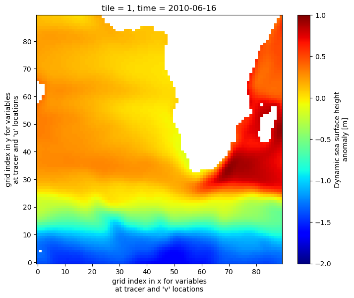
Let’s work on tile 1, time = 5 (June, 2010)

fig=plt.figure(figsize=(8, 6.5))

ecco_ds.SSH.isel(tile=1,time=5).plot(cmap='jet',vmin=-2, vmax=1)

<matplotlib.collections.QuadMesh at 0x1ce9771e970>

Subset tile 1, j = 50 (a single row through the array), and time = 5 (June 2010)

output_tile1_time06_j50= ecco_ds.isel(tile=1, time=5, j=50).load()
output_tile1_time06_j50.data_vars

Data variables:
    CS        (i) float32 1.0 1.0 1.0 1.0 1.0 1.0 ... 1.0 1.0 1.0 1.0 1.0 1.0
    SN        (i) float32 -3.751e-15 1.875e-15 ... -1.875e-15 3.751e-15
    rA        (i) float32 1.108e+10 1.108e+10 1.108e+10 ... 1.108e+10 1.108e+10
    dxG       (j_g, i) float32 6.054e+04 6.054e+04 ... 1.098e+05 1.098e+05
    dyG       (i_g) float32 1.055e+05 1.055e+05 ... 1.055e+05 1.055e+05
    Depth     (i) float32 3.343e+03 3.809e+03 4.016e+03 ... 4.404e+03 4.833e+03
    rAz       (j_g, i_g) float32 3.584e+09 3.584e+09 ... 1.179e+10 1.179e+10
    dxC       (i_g) float32 1.05e+05 1.05e+05 1.05e+05 ... 1.05e+05 1.05e+05
    dyC       (j_g, i) float32 5.92e+04 5.92e+04 ... 1.074e+05 1.074e+05
    rAw       (i_g) float32 1.108e+10 1.108e+10 ... 1.108e+10 1.108e+10
    rAs       (j_g, i) float32 3.584e+09 3.584e+09 ... 1.179e+10 1.179e+10
    drC       (k_p1) float32 5.0 10.0 10.0 10.0 10.0 ... 399.0 422.0 445.0 228.2
    drF       (k) float32 10.0 10.0 10.0 10.0 10.0 ... 387.5 410.5 433.5 456.5
    PHrefC    (k) float32 49.05 147.1 245.2 ... 4.944e+04 5.357e+04 5.794e+04
    PHrefF    (k_p1) float32 0.0 98.1 196.2 ... 5.145e+04 5.57e+04 6.018e+04
    hFacC     (k, i) float32 1.0 1.0 1.0 1.0 1.0 1.0 ... 0.0 0.0 0.0 0.0 0.0 0.0
    hFacW     (k, i_g) float32 1.0 1.0 1.0 1.0 1.0 1.0 ... 0.0 0.0 0.0 0.0 0.0
    hFacS     (k, j_g, i) float32 1.0 1.0 1.0 1.0 1.0 ... 0.0 0.0 0.0 0.0 0.0
    maskC     (k, i) bool True True True True True ... False False False False
    maskW     (k, i_g) bool True True True True True ... False False False False
    maskS     (k, j_g, i) bool True True True True ... False False False False
    SSH       (i) float32 0.31 0.328 0.3291 0.3225 ... nan 0.8263 0.8856 0.9166
    SSHIBC    (i) float32 -0.07849 -0.07787 -0.07717 ... -0.07901 -0.07715
    SSHNOIBC  (i) float32 0.2315 0.2502 0.2519 0.2462 ... 0.7423 0.8066 0.8394
    ETAN      (i) float32 0.2282 0.2468 0.2486 0.2429 ... 0.739 0.8033 0.8361
    OBP       (i) float32 20.13 27.04 30.4 32.93 33.83 ... nan 16.19 37.27 45.54
    OBPGMAP   (i) float32 30.16 37.06 40.43 42.95 ... nan 26.21 47.29 55.56
    PHIBOT    (i) float32 295.8 363.5 396.5 421.3 ... nan 257.1 463.9 545.0

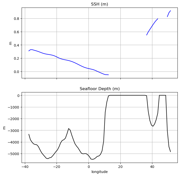
All variables that had tile, time, or j coordinates have been subset while other variables (including those with the offset j_g coordinates) are unchanged. Let’s plot the seafloor depth and sea surface height from west to east along j=50, (see plot at Line 16) which extends across the S. Atlantic, across Africa to Madagascar, and finally into to W. Indian Ocean.

f, axarr = plt.subplots(2, sharex=True,figsize=(8, 8))
(ax1, ax2) = axarr
ax1.plot(output_tile1_time06_j50.XC, output_tile1_time06_j50.SSH,color='b')
ax1.set_ylabel('m')
ax1.set_title('SSH (m)')
ax1.grid()

ax2.plot(output_tile1_time06_j50.XC, -output_tile1_time06_j50.Depth,color='k')
ax2.set_xlabel('longitude')
ax2.set_ylabel('m')
ax2.set_title('Seafloor Depth (m)')
ax2.grid()

Subsetting using the where( ) syntax

The where( ) method is quite different than other subsetting methods because subsetting is done by masking out values with nans that do not meet some specified criteria.

For more infomation about where( ) see http://xarray.pydata.org/en/stable/indexing.html#masking-with-where

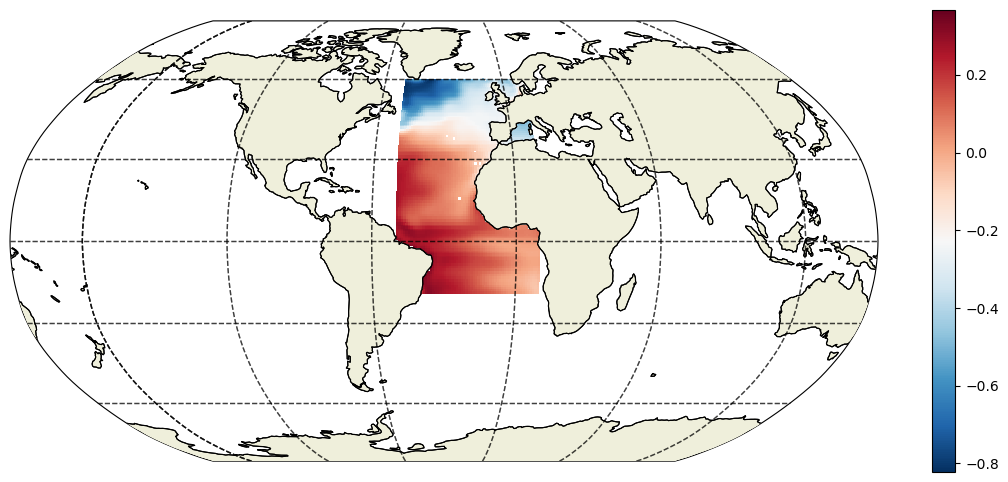
Let’s demonstrate where by masking out all SSH values that do not fall within a box defined between 20S to 60N and 50W to 10E.

First, we’ll extract the SSH DataArray

ssh_da=ecco_ds.SSH

Create a matrix that is True where latitude is between 20S and 60N and False otherwise.

lat_bounds = np.logical_and(ssh_da.YC  > -20, ssh_da.YC < 60)

Create a matrix that is True where longitude is between 50W and 10E and False otherwise.

lon_bounds = np.logical_and(ssh_da.XC  > -50, ssh_da.XC < 10)

Combine the lat_bounds and lon_bounds logical matrices:

lat_lon_bounds = np.logical_and(lat_bounds, lon_bounds)

Finally, use where to mask out all SSH values that do not fall within our lat_lon_bounds

ssh_da_subset_space = ssh_da.where(lat_lon_bounds, np.nan)

To visualize the SSH in our box we’ll use one of our ECCO v4 custom plotting routines (which will be the subject of another tutorial).

Notice the use of .sel( ) to subset a single time slice (time=1) for plotting.

fig=plt.figure(figsize=(14, 6))

ecco.plot_proj_to_latlon_grid(ecco_ds.XC, ecco_ds.YC, \
                              ssh_da_subset_space.isel(time=6),\
                              dx=.5, dy=.5,user_lon_0 = -30,\
                              show_colorbar=True);

-179.75 149.75
-180.0 150.0
-89.75 89.75
-90.0 90.0
150.25424720338984 179.74576279661017
150.00001 180.0
-89.75 89.75
-90.0 90.0

Conclusion

You now know several different methods for accessing and subsetting fields in Dataset and DataArray objects.

To learn a more about indexing/subsetting methods please refer to the xarray manual for indexing methods, http://xarray.pydata.org/en/stable/indexing.html.