Compute meridional heat transport
This notebook shows how to compute meridional heat transport (MHT) across any particular latitude band. Additionally, we show this for both global and basin specific cases.
Oceanographic computations:
use xgcm to compute masks and grab values at a particular latitude band
use ecco_v4_py to select a specific basin
compute meridional heat transport at one or more latitude bands
Python basics on display:
how to open a dataset using xarray (a one liner!)
how to save a dataset using xarray (another one liner!)
one method for making subplots
some tricks for plotting quantities defined as dask arrays
Note that each of these tasks can be accomplished more succinctly with ecco_v4_py functions, but are shown explicitly to illustrate these tools. Throughout, we will note the ecco_v4_py (python) and gcmfaces (MATLAB) functions which can perform these computations.
Datasets
These are the ShortNames of the ECCO datasets needed for this tutorial:
ECCO_L4_GEOMETRY_LLC0090GRID_V4R4
ECCO_L4_OCEAN_3D_TEMPERATURE_FLUX_LLC0090GRID_MONTHLY_V4R4 (1992-2017)
Make sure you have the ecco_access package before you run this tutorial. It will handle the access to the datasets (either in-cloud access from S3 or Internet download, depending on the incloud_access option you specify).
[33]:
import warnings
warnings.filterwarnings('ignore')
[34]:
import os
import matplotlib.pyplot as plt
import numpy as np
import xarray as xr
import cartopy as cart
import sys
import glob

from os.path import join,expanduser,exists,split
user_home_dir = expanduser('~')


import ecco_v4_py as ecco
import ecco_access as ea


# are you working in the AWS Cloud?
incloud_access = False

# indicate mode of access from PO.DAAC
# options are:
# 'download': direct download from internet to your local machine
# 'download_ifspace': like download, but only proceeds
#                     if your machine have sufficient storage
# 's3_open': access datasets in-cloud from an AWS instance
# 's3_open_fsspec': use jsons generated with fsspec and
#                   kerchunk libraries to speed up in-cloud access
# 's3_get': direct download from S3 in-cloud to an AWS instance
# 's3_get_ifspace': like s3_get, but only proceeds if your instance
#                   has sufficient storage
user_home_dir = expanduser('~')
download_dir = join(user_home_dir,'Downloads','ECCO_V4r4_PODAAC')
if incloud_access:
    access_mode = 's3_open_fsspec'
    download_root_dir = None
    jsons_root_dir = join(user_home_dir,'MZZ')
else:
    access_mode = 'download_ifspace'
    download_root_dir = download_dir
    jsons_root_dir = None
Since we will be dealing with large datasets spanning the full depth of the ocean and time span of ECCO, let’s make use of dask’s cluster capabilities as well.
[35]:
# setting up a dask LocalCluster
from dask.distributed import Client
from dask.distributed import LocalCluster
cluster = LocalCluster()
client = Client(cluster)
client
[35]:
Client
Client-f173ef33-8ccc-11ef-a5db-ea833bf36b53
| Connection method: Cluster object | Cluster type: distributed.LocalCluster |
| Dashboard: http://127.0.0.1:43073/status |
Cluster Info
LocalCluster
d7112729
| Dashboard: http://127.0.0.1:43073/status | Workers: 4 |
| Total threads: 4 | Total memory: 15.27 GiB |
| Status: running | Using processes: True |
Scheduler Info
Scheduler
Scheduler-e2829a07-e5e3-4e89-ba5b-a1a408de3ebe
| Comm: tcp://127.0.0.1:46407 | Workers: 4 |
| Dashboard: http://127.0.0.1:43073/status | Total threads: 4 |
| Started: Just now | Total memory: 15.27 GiB |
Workers
Worker: 0
| Comm: tcp://127.0.0.1:38215 | Total threads: 1 |
| Dashboard: http://127.0.0.1:33409/status | Memory: 3.82 GiB |
| Nanny: tcp://127.0.0.1:43449 | |
| Local directory: /tmp/dask-scratch-space/worker-_ghajqtc | |
Worker: 1
| Comm: tcp://127.0.0.1:37585 | Total threads: 1 |
| Dashboard: http://127.0.0.1:42657/status | Memory: 3.82 GiB |
| Nanny: tcp://127.0.0.1:39359 | |
| Local directory: /tmp/dask-scratch-space/worker-u_eawi3w | |
Worker: 2
| Comm: tcp://127.0.0.1:36829 | Total threads: 1 |
| Dashboard: http://127.0.0.1:35033/status | Memory: 3.82 GiB |
| Nanny: tcp://127.0.0.1:34019 | |
| Local directory: /tmp/dask-scratch-space/worker-gwfpkxia | |
Worker: 3
| Comm: tcp://127.0.0.1:39379 | Total threads: 1 |
| Dashboard: http://127.0.0.1:44403/status | Memory: 3.82 GiB |
| Nanny: tcp://127.0.0.1:42287 | |
| Local directory: /tmp/dask-scratch-space/worker-ft_mo4_k | |
Load Model Variables
Because we’re computing transport, we want the files containing ‘UVELMASS’ and ‘VVELMASS’ for volumetric transport, and ‘ADVx_TH’, ‘ADVy_TH’ and ‘DFxE_TH’, ‘DFyE_TH’ for the advective and diffusive components of heat transport, respectively.
[6]:
## Access datasets needed for this tutorial

ShortNames_list = ["ECCO_L4_GEOMETRY_LLC0090GRID_V4R4",\
                   "ECCO_L4_OCEAN_3D_TEMPERATURE_FLUX_LLC0090GRID_MONTHLY_V4R4"]
StartDate = '1992-01'
EndDate = '2017-12'
ds_dict = ea.ecco_podaac_to_xrdataset(ShortNames_list,\
                                            StartDate=StartDate,EndDate=EndDate,\
                                            mode=access_mode,\
                                            download_root_dir=download_root_dir,\
                                            jsons_root_dir=jsons_root_dir,\
                                            max_avail_frac=0.5)
[7]:
## Open the model grid
ecco_grid = ds_dict[ShortNames_list[0]].chunk({'k':50,'tile':13,'j':90,'j_g':90,'i':90,'i_g':90})

## Create a dataset of monthly advective and diffusive temperature fluxes, 1992-2017
ecco_vars = ds_dict[ShortNames_list[1]].chunk({'k':50,'tile':13,'j':90,'j_g':90,'i':90,'i_g':90})

## Drop the vertical temperature fluxes as we only need horizontal fluxes to compute MHT
ecco_vars = ecco_vars.drop_vars(['ADVr_TH','DFrE_TH','DFrI_TH'])

## Merge the ecco_grid with the ecco_vars to make the ecco_ds
ecco_ds = xr.merge((ecco_grid , ecco_vars))
Grab latitude band: 26 N array as an example
Here we want to grab the transport values which along the band closest represented in the model to 26N. In a latitude longitude grid this could simply be done by, e.g. U.sel(lat=26). However, the LLC grid is slightly more complicated. Luckily, the functionality enabled by the xgcm Grid object makes this relatively easy.
Note that this subsection can be performed with the with the ecco_v4_py modules vector_calc and scalar_calc as follows:
from ecco_v4_py import vector_calc, scalar_calc
grid = ecco_v4_py.get_llc_grid(ds)
rapid_maskW, rapid_maskS = vector_calc.get_latitude_masks(lat_val=26,yc=ds.YC,grid=grid)
rapid_maskC = scalar_calc.get_latitude_mask(lat_val=26,yc=ds.YC,grid=grid)
One can also use the gcmfaces function gcmfaces_calc/gcmfaces_lines_zonal.m.
[8]:
# Get array of 1's at and north of latitude
lat = 26
ones = xr.ones_like(ecco_ds.YC)
dome_maskC = ones.where(ecco_ds.YC>=lat,0).compute()
[9]:
plt.figure(figsize=(12,6))
ecco.plot_proj_to_latlon_grid(ecco_ds.XC,ecco_ds.YC,dome_maskC,
                              projection_type='robin',cmap='viridis',user_lon_0=0,show_colorbar=True);
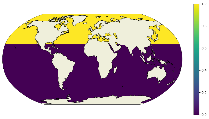
Again, if this were a lat/lon grid we could simply take a finite difference in the meridional direction. The only grid cells with 1’s remaining would be at the southern edge of grid cells at approximately 26N.
However, recall that the LLC grid has a different picture.
[10]:
maskC = ecco_ds.maskC.compute()
maskS = ecco_ds.maskS.compute()
maskW = ecco_ds.maskW.compute()
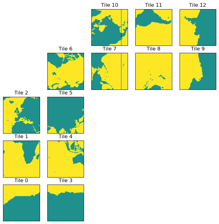
[11]:
plt.figure(figsize=(12,6))
ecco.plot_tiles(dome_maskC+maskC.isel(k=0), cmap='viridis');
<Figure size 1200x600 with 0 Axes>

Recall that for tiles 7-12, the y-dimension actually runs East-West. Therefore, we want to compute a finite difference in the x-dimension on these tiles to get the latitude band at 26N. For tiles 1-5, we clearly want to difference in the y-dimension. Things get more complicated on tile 6.
Here we make the xgcm Grid object which allows us to compute finite differences in simple one liners. This object understands how each of the tiles on the LLC grid connect, because we provide that information. To see under the hood, checkout the utility function get_llc_grid where these connections are defined.
[12]:
grid = ecco.get_llc_grid(ecco_ds)
[13]:
lat_maskW = grid.diff(dome_maskC,'X',boundary='fill')
lat_maskS = grid.diff(dome_maskC,'Y',boundary='fill')
[14]:
plt.figure(figsize=(12,6))
ecco.plot_tiles(lat_maskW+maskW.isel(k=0), cmap='viridis');
<Figure size 1200x600 with 0 Axes>
[15]:
plt.figure(figsize=(12,6))
ecco.plot_tiles(lat_maskS+maskS.isel(k=0), cmap='viridis',show_colorbar=True);
<Figure size 1200x600 with 0 Axes>

Select the Atlantic ocean basin for RAPID-MOCHA MHT
Now that we have 26N we just need to select the Atlantic. This can be done with the ecco_v4_py.get_basin module, specifically ecco_v4_py.get_basin.get_basin_mask. Note that this function requires a mask as an input, and then returns the values within a particular ocean basin. Therefore, provide the function with ds['maskC'] for a mask at tracer points, ds['maskW'] for west grid cell
edges, etc.
Note: this mirrors the gcmfaces functionality ecco_v4/v4_basin.m.
Here we just want the Atlantic ocean, but lets look at what options we have …
[16]:
print(ecco.get_available_basin_names())
['pac', 'atl', 'ind', 'arct', 'bering', 'southChina', 'mexico', 'okhotsk', 'hudson', 'med', 'java', 'north', 'japan', 'timor', 'eastChina', 'red', 'gulf', 'baffin', 'gin', 'barents']
Notice that, for instance, ‘mexico’ exists separately from the Atlantic (‘atl’). This is to provide as fine granularity as possible (and sensible). To grab the broader Atlantic ocean basin, i.e. the one people usually refer to, use the option ‘atlExt’. Similar options exist for the Pacific and Indian ocean basins.
[17]:
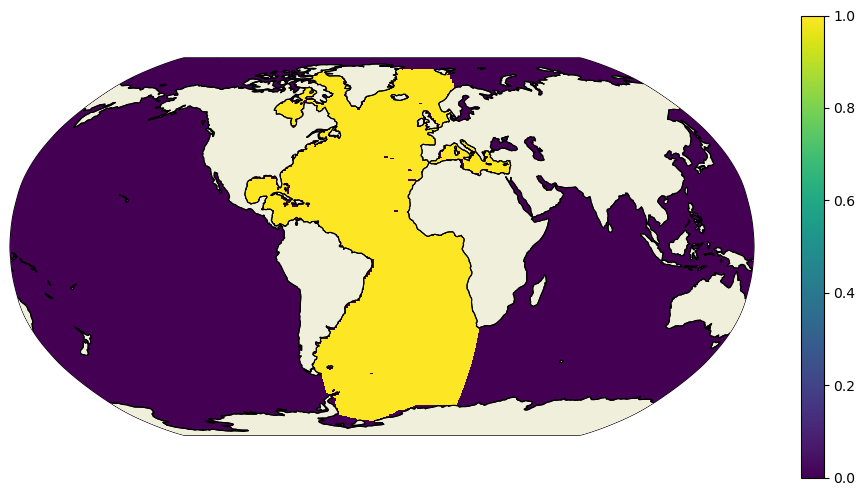
try:
    atl_maskW = ecco.get_basin_mask(basin_name='atlExt',mask=maskW.isel(k=0))
    atl_maskS = ecco.get_basin_mask(basin_name='atlExt',mask=maskS.isel(k=0))
except:
    # depending on how ecco_v4_py is downloaded/installed,
    # the basin mask file may not be in the location expected by ecco_v4_py.
    # This will download the file from the ECCOv4-py GitHub online.
    basin_path = join(user_home_dir,'ECCOv4-py','binary_data')
    if exists(join(basin_path,'basins.data')) == False:
        import requests
        url_basin_mask = "https://github.com/ECCO-GROUP/ECCOv4-py/raw/master/binary_data/basins.data"
        source_file = requests.get(url_basin_mask, allow_redirects=True)
        if exists(basin_path) == False:
            os.makedirs(basin_path)
        target_file = open(join(basin_path,'basins.data'),'wb')
        target_file.write(source_file.content)
    atl_maskW = ecco.get_basin_mask(basin_name='atlExt',mask=maskW.isel(k=0),\
                                    basin_path=basin_path)
    atl_maskS = ecco.get_basin_mask(basin_name='atlExt',mask=maskS.isel(k=0),\
                                    basin_path=basin_path)
get_basin_name:  ['atl', 'mexico', 'hudson', 'med', 'north', 'baffin', 'gin'] /srv/conda/envs/notebook/lib/python3.11/site-packages/binary_data
get_basin_name:  ['atl', 'mexico', 'hudson', 'med', 'north', 'baffin', 'gin'] /home/jovyan/ECCOv4-py/binary_data
load_binary_array: loading file /home/jovyan/ECCOv4-py/binary_data/basins.data
load_binary_array: data array shape  (1170, 90)
load_binary_array: data array type  >f4
llc_compact_to_faces: dims, llc  (1170, 90) 90
llc_compact_to_faces: data_compact array type  >f4
llc_faces_to_tiles: data_tiles shape  (13, 90, 90)
llc_faces_to_tiles: data_tiles dtype  >f4
shape after reading
(13, 90, 90)
Notice that we pass the routine a 2D mask by selecting the first depth level. This is simply to make things run faster.
[18]:
plt.figure(figsize=(12,6))
ecco.plot_proj_to_latlon_grid(ecco_ds.XC,ecco_ds.YC,atl_maskW,
                              projection_type='robin',cmap='viridis',user_lon_0=-30,show_colorbar=True);
MHT at the approximate RAPID array latitude
This can be done with the ecco_v4_py.calc_meridional_trsp module for heat, salt, and volume transport as follows:
mvt = ecco_v4_py.calc_meridional_vol_trsp(ecco_ds,lat_vals=26,basin_name='atlExt')
mht = ecco_v4_py.calc_meridional_heat_trsp(ecco_ds,lat_vals=26,basin_name='atlExt')
mst = ecco_v4_py.calc_meridional_salt_trsp(ecco_ds,lat_vals=26,basin_name='atlExt')
Additionally, one could compute the overturning streamfunction at this latitude band with ecco_v4_py.calc_meridional_stf. The inputs are the same as the functions above, see the module ecco_v4_py.calc_stf.
In MATLAB, one can use the functions:
compute meridional transports: gcmfaces_calc/calc_MeridionalTransport.m
compute the overturning streamfunction: gcmfaces_calc/calc_overturn.m
A note about computational performance
When we originally open the dataset with all of the variables, we don’t actually load anything into memory. In fact, nothing actually happens until “the last minute”. For example, the data are only loaded once we do any computation like compute a mean value, plot something, or explicitly provide a load command for either the entire dataset or an individual DataArray within the dataset. This ‘lazy execution’ is enabled by the data structure underlying the xarray Datasets and DataArrays, the
dask array.
In short, the when the data are opened, dask builds an execution task graph which it saves up to execute at the last minute. Dask also allows for parallelism, and by default runs in parallel across threads for a single core architecture. For now, this is what we will show.
Some quick tips are:
Don’t load the full 26 years of ECCOv4r4 output (e.g., the
ecco_dsdataset in this notebook) unless you’re on a machine with plenty of memory.If you’re in this situation where you can’t load all months into memory, it’s a good idea to load a final result before plotting, in case you need to plot it many times in a row, see below…
To illustrate the memory savings from dask, let’s see the footprint of loading a single year of ecco_ds into memory:
[36]:
%%time

from pympler import asizeof
# function to quantify memory footprint of a dataset
def memory_footprint(ds):
    s = 0
    for i in list(ds.keys()):
        s += asizeof.asizeof(ds[i].compute())
    return s


# Create a deep copy of one year (2000) of ecco_ds
ecco_ds_2000 = (ecco_ds.isel(time=np.logical_and(ecco_ds.time.values >= np.datetime64('2000-01-01','ns'),\
                                                ecco_ds.time.values < np.datetime64('2001-01-01','ns')))\
               ).copy(deep=True)

# quantify in-memory footprint
memory_footp = memory_footprint(ecco_ds_2000)

print('Memory footprint: ' + str(memory_footp/(2**20)) + ' MB')
Memory footprint: 1135.168571472168 MB
CPU times: user 1.49 s, sys: 756 ms, total: 2.24 s
Wall time: 12.2 s
The memory footprint of one year of ecco_ds is >1 GB. If we loaded all 26 years into memory this could be a problem on a personal laptop. But with dask, we can delay loading these fields into memory, and when we do the computations they are handled in chunks.
[20]:
%%time

# Compute MHT in Atlantic basin
trsp_x = ((ecco_ds['ADVx_TH'] + ecco_ds['DFxE_TH']) *  atl_maskW).sum('k')
trsp_y = ((ecco_ds['ADVy_TH'] + ecco_ds['DFyE_TH']) *  atl_maskS).sum('k')

## Quantify memory footprint of fields involved
def sum_memory_footprint(da_list):
    memory_footp = 0
    for da in da_to_sum_memory:
        memory_footp += asizeof.asizeof(eval(da))
    return memory_footp

da_to_sum_memory = ["ecco_ds['ADVx_TH']","ecco_ds['DFxE_TH']","atl_maskW","trsp_x",\
                    "ecco_ds['ADVy_TH']","ecco_ds['DFyE_TH']","atl_maskS","trsp_y"]
memory_footp = sum_memory_footprint(da_to_sum_memory)

print('Memory footprint: ' + str(memory_footp/(2**20)) + ' MB')
Memory footprint: 517.7715225219727 MB
CPU times: user 3.34 s, sys: 302 ms, total: 3.64 s
Wall time: 3.63 s
[21]:
%%time

# Apply latitude mask
trsp_x = trsp_x * lat_maskW
trsp_y = trsp_y * lat_maskS

# Sum horizontally
trsp_x = trsp_x.sum(dim=['i_g','j','tile'])
trsp_y = trsp_y.sum(dim=['i','j_g','tile'])

# Add together to get transport
trsp = trsp_x + trsp_y

# Convert to PW
mht = trsp * (1.e-15 * 1000 * 4000)
mht.attrs['units']='PW'


## Quantify memory footprint of fields involved
da_to_sum_memory = ["trsp_x","lat_maskW","trsp_y","lat_maskS","trsp","mht"]
memory_footp = sum_memory_footprint(da_to_sum_memory)

print('Memory footprint: ' + str(memory_footp/(2**20)) + ' MB')
Memory footprint: 338.3598327636719 MB
CPU times: user 2.16 s, sys: 230 ms, total: 2.39 s
Wall time: 2.36 s
Now that we have computed MHT, lets load the result for iterative plotting
For some reason when dask arrays are plotted, they are computed on the spot but don’t stay in memory. This takes a bit to get the hang of, but keep in mind that this allows us to scale the same code on distributed architecture, so we could use these same routines for high resolution output. This seems worthwhile!
Note that we probably don’t need this load statement if we have already loaded the underlying datasets.
[22]:
%%time
# Load mht DataArray into memory.
# The script below is a more complex version of mht = mht.compute(),
# but it works more consistently in memory-limited environments
mht_inmemory = np.empty(mht.shape)
for t in range(mht.sizes['time']):
    mht_inmemory[t] = mht[t].compute()
mht_da = xr.DataArray(data=mht_inmemory,dims=mht.dims,coords=mht.coords,attrs=mht.attrs)
del mht
mht = mht_da
CPU times: user 50.5 s, sys: 7.53 s, total: 58 s
Wall time: 9min 23s
[23]:
%%time
plt.figure(figsize=(12,6))
plt.plot(mht['time'],mht,'r')
plt.grid()
plt.title('Monthly Meridional Heat Transport at 26N')
plt.ylabel(f'[{mht.attrs["units"]}]')
plt.show()

CPU times: user 173 ms, sys: 13.3 ms, total: 186 ms
Wall time: 169 ms
Now compare global and Atlantic MHT at many latitudes
[24]:
mht
[24]:
<xarray.DataArray (time: 312)> Size: 2kB
array([0.62334746, 0.80589411, 1.04600461, 0.94122674, 0.90720813,
       0.80292317, 1.0488881 , 1.211121  , 1.15382551, 0.90893692,
       1.44971909, 1.02674969, 1.12807911, 0.73802931, 0.83042615,
       0.85161099, 0.80667569, 0.82807073, 0.92744497, 0.97638034,
       1.05139303, 0.75934727, 1.36689865, 1.07707478, 1.40224997,
       1.00816617, 0.99943306, 0.96495009, 0.82479508, 0.78128435,
       1.05446313, 1.06591878, 0.90124748, 0.77375916, 1.07170695,
       0.95836544, 1.02515503, 0.81284626, 0.72586811, 0.67142316,
       0.5820906 , 0.66141199, 0.9382528 , 0.94098504, 0.82740239,
       0.94309232, 0.93982565, 0.63365516, 0.7962627 , 0.78199906,
       0.59654641, 0.73988101, 0.73155197, 0.86845564, 1.01992155,
       1.05562354, 0.8971817 , 0.77888028, 1.13842791, 0.6051433 ,
       0.69298914, 1.1883513 , 0.80078545, 0.4866397 , 0.66300679,
       0.54972587, 0.85218995, 0.874945  , 0.76988568, 0.66923101,
       0.90993869, 0.64036485, 0.97607703, 0.34217713, 0.93760614,
       0.79087747, 0.57711653, 0.68861999, 1.06454401, 1.18294696,
       0.86147057, 0.96079199, 1.00166426, 1.27482262, 1.1541138 ,
       0.78456649, 0.65456561, 0.68231101, 0.56033296, 0.82880318,
       0.87628208, 0.92605802, 0.92296105, 1.01064977, 1.06934463,
       0.86133597, 0.88730193, 0.90410428, 0.57923081, 0.72182206,
...
       0.46761163, 0.36275844, 0.08466888, 0.28339223, 0.50880637,
       0.70170707, 0.9730668 , 1.03992566, 0.91965565, 1.10777821,
       0.97123405, 0.64935843, 0.16917321, 0.65066321, 0.80998092,
       0.7061887 , 0.89771864, 0.59762354, 0.70094349, 0.96033755,
       0.92052749, 0.90165742, 1.0177366 , 0.90706611, 1.22864268,
       0.87870624, 0.77473163, 0.94509074, 0.65740948, 0.57038699,
       0.48089773, 0.94304844, 0.86842176, 0.61943532, 0.62843399,
       0.84385346, 0.93570686, 0.73939602, 0.69129776, 0.09529923,
       0.64611389, 0.7745165 , 0.93955469, 0.88589726, 1.03218635,
       0.78964431, 0.73128252, 0.91007758, 1.03144186, 1.07448102,
       0.9411615 , 0.72365324, 0.56716582, 0.72720107, 0.69900984,
       0.73430012, 0.76954193, 0.64122061, 0.63719108, 0.95265634,
       0.86030805, 1.01866351, 0.8128125 , 0.921338  , 0.63231767,
       0.7516123 , 0.73238916, 0.85881188, 0.85381196, 0.72003521,
       0.73323922, 1.01775801, 1.00338291, 0.56101913, 0.95687684,
       0.6906106 , 0.53181503, 0.65913571, 0.69513319, 1.01599762,
       0.91846464, 1.01359296, 0.84206591, 0.94374317, 0.95176903,
       0.74324589, 0.73401651, 0.94528062, 0.59728757, 0.61301111,
       0.82555021, 1.08339009, 0.98624291, 0.8755259 , 0.8440195 ,
       0.81200697, 0.90053641])
Coordinates:
  * time     (time) datetime64[ns] 2kB 1992-01-16T18:00:00 ... 2017-12-16T06:...
Attributes: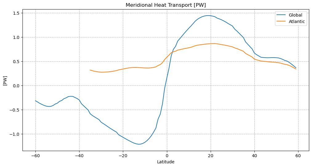
units: PWHere we will compute MHT along a number of latitudes, integrated both globally and in the Atlantic basin only, and plot the result.
[25]:
%%time

global_lats = np.arange(-60,60,1)
atl_lats = np.arange(-35,60,1)

## The ecco_v4_py function below does the work of computing MHT at a number of latitudes in a single line.
## However, for large datasets (e.g. 26 years of full-depth global output) it is very slow on a laptop.

# curr_mht = ecco.calc_meridional_heat_trsp(ecco_ds,lat_vals=global_lats)
# curr_mht = curr_mht.mean('time')

## This code runs faster for some reason, perhaps due to the way the latitude masking is done.

ecco_YC = ecco_ds.YC.compute()
trsp_tmean_x = (ecco_ds['ADVx_TH'] + ecco_ds['DFxE_TH']).mean('time')
trsp_tmean_y = (ecco_ds['ADVy_TH'] + ecco_ds['DFyE_TH']).mean('time')
trsp_x = trsp_tmean_x.where(ecco_ds.maskW).compute()
trsp_y = trsp_tmean_y.where(ecco_ds.maskS).compute()

global_trsp_z = np.empty((ecco_ds.dims['k'],len(global_lats)))
atl_trsp_z = np.empty((ecco_ds.dims['k'],len(atl_lats)))
atl_count = 0
for count,lat in enumerate(global_lats):
    dome_maskC = (ecco_YC >= lat).astype('float')
    lat_maskW = grid.diff(dome_maskC,'X',boundary='fill')
    lat_maskS = grid.diff(dome_maskC,'Y',boundary='fill')
    trsp_x_atlat = (trsp_x * lat_maskW).sum(dim=['tile','j','i_g'])
    trsp_y_atlat = (trsp_y * lat_maskS).sum(dim=['tile','j_g','i'])
    global_trsp_z[:,count] = (trsp_x_atlat + trsp_y_atlat).values

    if lat in atl_lats:
        trsp_x_atlat_Atl = (trsp_x * lat_maskW * atl_maskW).sum(dim=['tile','j','i_g'])
        trsp_y_atlat_Atl = (trsp_y * lat_maskS * atl_maskS).sum(dim=['tile','j_g','i'])
        atl_trsp_z[:,atl_count] = (trsp_x_atlat_Atl + trsp_y_atlat_Atl).values
        atl_count += 1

    if count % 10 == 0:
        print('Computed MHT up through ' + str(lat) + ' deg lat')


# convert temperature flux to heat transport
global_trsp_z = global_trsp_z*(1.e-15 * 1000 * 4000)
atl_trsp_z = atl_trsp_z*(1.e-15 * 1000 * 4000)

# create DataArrays from Numpy arrays generated in the above loop
global_heat_trsp_z = xr.DataArray(global_trsp_z,\
                                  dims=['k','lat'],\
                                  coords={'Z':(['k'],ecco_ds.Z.data),'lat':global_lats},\
                                 )
global_heat_trsp_z['Z'] = ecco_ds['Z']    # include attributes of Z from ecco_ds
global_heat_trsp_z.attrs['units']='PW'
atl_heat_trsp_z = xr.DataArray(atl_trsp_z,\
                                  dims=['k','lat'],\
                                  coords={'Z':(['k'],ecco_ds.Z.data),'lat':atl_lats},\
                              )
atl_heat_trsp_z['Z'] = ecco_ds['Z']
atl_heat_trsp_z.attrs['units']='PW'
global_heat_trsp = global_heat_trsp_z.sum('k')
global_heat_trsp.attrs['units']='PW'
atl_heat_trsp = atl_heat_trsp_z.sum('k')
atl_heat_trsp.attrs['units']='PW'
Computed MHT up through -60 deg lat
Computed MHT up through -50 deg lat
Computed MHT up through -40 deg lat
Computed MHT up through -30 deg lat
Computed MHT up through -20 deg lat
Computed MHT up through -10 deg lat
Computed MHT up through 0 deg lat
Computed MHT up through 10 deg lat
Computed MHT up through 20 deg lat
Computed MHT up through 30 deg lat
Computed MHT up through 40 deg lat
Computed MHT up through 50 deg lat
CPU times: user 23.2 s, sys: 6.7 s, total: 29.9 s
Wall time: 1min 47s
[26]:
# create dataset containing global and Atlantic MHT, and save as NetCDF file
mht = global_heat_trsp_z.to_dataset(name='global_heat_trsp_z')
atl = atl_heat_trsp_z.to_dataset(name='atl_heat_trsp_z')
mht['global_heat_trsp'] = global_heat_trsp
atl['atl_heat_trsp'] = atl_heat_trsp

# pick a temp directory for yourself to save file
nc_save_dir = join(user_home_dir,'Downloads')

if not os.path.isdir(nc_save_dir):
    os.makedirs(nc_save_dir)

nc_file = f'{nc_save_dir}/ecco_mht.nc'

ds_mht = xr.merge((mht,atl))
ds_mht.to_netcdf(nc_file)            # save dataset as NetCDF file
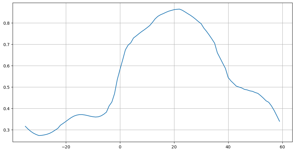
[27]:
plt.figure(figsize=(12,6))
plt.plot(mht['lat'], mht['global_heat_trsp'])
plt.grid();
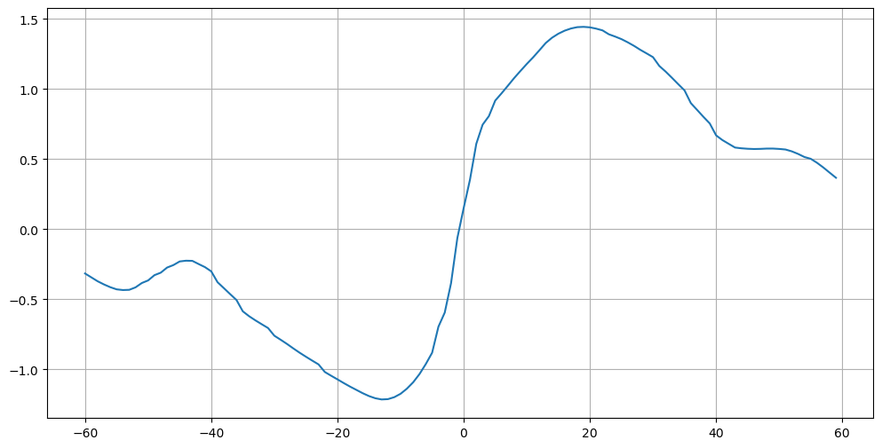
[28]:
plt.figure(figsize=(12,6))
plt.plot(atl['lat'], atl['atl_heat_trsp'])
plt.grid()
[29]:
plt.figure(figsize=(12,6))
plt.plot(mht['lat'], mht['global_heat_trsp'])
plt.plot(atl['lat'], atl['atl_heat_trsp'])
plt.legend(('Global','Atlantic'))
plt.grid(linestyle='--')
plt.title(f'Meridional Heat Transport [{mht["global_heat_trsp"].attrs["units"]}]')
plt.ylabel(f'[{mht["global_heat_trsp"].attrs["units"]}]')
plt.xlabel('Latitude')
plt.show()
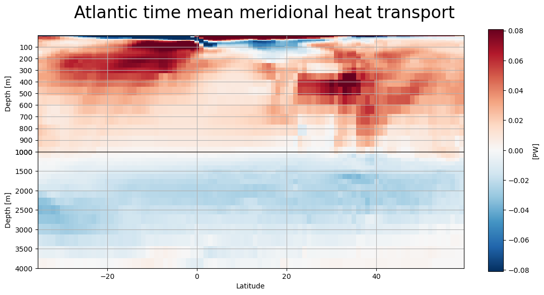
MHT as a function of depth
[30]:
def lat_depth_plot(mht,field,label):
    fig = plt.figure(figsize=(12,6))

    # Set up depth coordinate
    depth = -mht['Z']
    stretch_depth = 1000

    # Set up colormap and colorbar
    cmap = 'RdBu_r'
    fld = mht[field]
    abs_max = np.max(np.abs([fld.min(),fld.max()]))
    cmin = -abs_max*.1
    cmax = -cmin

    # First the "stretched" top plot
    ax1 = plt.subplot(2,1,1)
    p1 = ax1.pcolormesh(mht['lat'],depth,fld,cmap=cmap,vmin=cmin,vmax=cmax)
    plt.grid()

    # Handle y-axis
    ax1.invert_yaxis()
    plt.ylim([stretch_depth, 0])
    ax1.yaxis.axes.set_yticks(np.arange(stretch_depth,0,-100))
    plt.ylabel(f'Depth [{mht["Z"].attrs["units"]}]')

    # Remove top plot xtick label
    ax1.xaxis.axes.set_xticklabels([])

    # Now the rest ...
    ax2 = plt.subplot(2,1,2)
    p2 = ax2.pcolormesh(mht['lat'],depth, fld, cmap=cmap,vmin=cmin,vmax=cmax)
    plt.grid()

    # Handle y-axis
    ax2.invert_yaxis()
    plt.ylim([4000, 1000])
    #yticks = np.flip(np.arange(6000,stretch_depth,-1000))
    #ax2.yaxis.axes.set_yticks(yticks)
    plt.ylabel(f'Depth [{mht["Z"].attrs["units"]}]')

    # Label  axis
    plt.xlabel('Latitude')

    # Reduce space between subplots
    fig.subplots_adjust(hspace=0.0)

    # Make a single title
    fig.suptitle(f'{label} time mean meridional heat transport',verticalalignment='top',fontsize=24)

    # Make an overyling colorbar
    fig.subplots_adjust(right=0.83)
    cbar_ax = fig.add_axes([0.87, 0.1, 0.025, 0.8])
    fig.colorbar(p2,cax=cbar_ax)
    cbar_ax.set_ylabel(f'[{mht[field].attrs["units"]}]')

    plt.show()
[31]:
lat_depth_plot(mht,'global_heat_trsp_z','Global')
lat_depth_plot(atl,'atl_heat_trsp_z','Atlantic')
2024-10-17 21:13:45,582 - distributed.client - WARNING - Couldn't gather 1 keys, rescheduling (('neg-86dcf2529d5c1248c34d8e9cb3e72522', 0),)

Exercise: reproduce figure from (Ganachaud and Wunsch, 2000)
[32]:
from IPython.display import Image
Image('../figures/ganachaud_mht.png')
[32]:
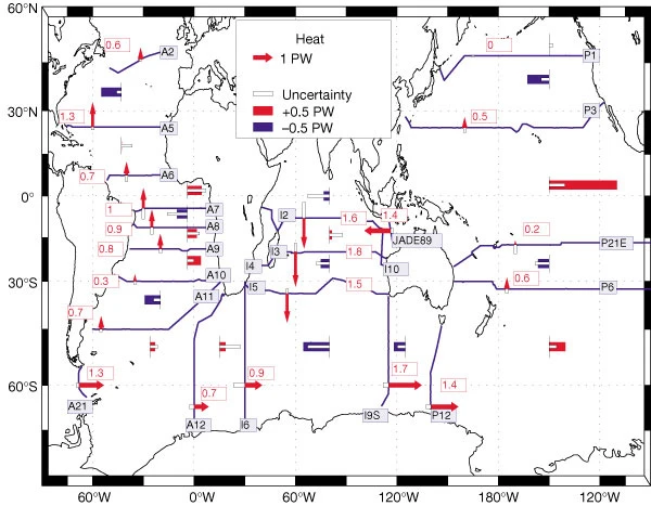
Note: to reproduce this figure, you may need to pair latitude masks with those defined through the get_section_masks module. An example of this functionality is shown in the next tutorial.
References
Ganachaud, A., & Wunsch, C. (2000). Improved estimates of global ocean circulation, heat transport and mixing from hydrographic data. Nature, 408(6811), 453-7. doi:http://dx.doi.org.ezproxy.lib.utexas.edu/10.1038/35044048