AWS Cloud: getting started and retrieving ECCO datasets

Andrew Delman, updated 2024-03-18.

Introduction

Previous tutorials have discussed how to download ECCO datasets from PO.DAAC to your local machine. However, during 2021-2022 PO.DAAC datasets (including ECCO) migrated to the NASA Earthdata Cloud hosted by Amazon Web Services (AWS). While data downloads from the cloud (using wget, curl, Python requests, etc.) function like downloads from any other website, there are definite advantages to working with datasets within the cloud environment. Data can be opened in an S3 bucket and viewed without downloading, or can be quickly downloaded to a user’s cloud instance for computations. For more information on PO.DAAC datasets in the cloud, there are a number of infographics here.

This tutorial will walk through the steps of how a user can set up an AWS instance and access ECCO datasets for computations in that instance. No prior experience with the AWS cloud is assumed.

Set up an AWS cloud instance

Computations in the AWS Cloud are typically done in an Amazon Elastic Compute Cloud (EC2) instance, which is a self-contained computing environment like the operating system on your local machine. You start an EC2 instance through the AWS Cloud management console, then connect to the instance (e.g., through ssh) like you would to any other machine, install the software that you need, and start working. AWS offers a Free Tier that provides 750 compute hours per month, 1 GB memory, and up to 30 GB storage for a period of 12 months. This is great for experimenting, but these memory/storage limits can be quite restrictive, so if you have institutional or project support for larger instances it is highly recommended to use them.

The steps here mostly follow this excellent tutorial on the PO.DAAC Cookbook.

Step 1: Create an AWS account

If you don’t already have one, create an account on AWS. Anyone with an e-mail address and a credit card can do this, though for the reasons above it is recommended that you seek out institutional support if possible, or include cloud computing costs in your grant proposals.

Step 2: Start an EC2 instance

Note: if you have an AWS account through the Jet Propulsion Laboratory (JPL), you will need to do Steps 2 and 3 differently. Please consult these instructions.

Once you log in to your new account, you should be at a screen with the title Console Home. First, let’s make sure you are in the most optimal AWS “region” for accessing PO.DAAC datasets, which are hosted in region us-west-2 (Oregon). In the upper-right corner of the page just to the left of your username, there is a drop-down menu with a place name on it. Select the US West (Oregon) us-west-2 region.

Now let’s start a new EC2 instance. Click on Services in the upper-left corner next to the AWS logo, then Compute –> EC2. On this new screen where there are a number of boxes, select the yellow Launch instance button. There are some settings on this screen to configure before launching the new instance:

Name and tags: Whatever you want (e.g., ECCO tutorials).

Application and OS images (Amazon Machine Image): Quick Start –> Red Hat –> Red Hat Enterprise Linux 9, SSD Volume Type This is not the only AMI you can use, and your institution may have preferred or required AMIs to use AWS cloud services. Make sure that the AMI you select runs Linux, and is “Free tier eligible” if you are not supported by your institution or project.

Instance type: t2.micro if using the Free tier. If you’re not restricted to the free tier, a t2.medium/t3.medium or larger is recommended. (t3 is a newer generation, with similar or slightly cheaper costs as t2.)

Key pair (login): Click on Create new key pair. In the pop-up window, make the name whatever you want (e.g., aws_ec2_jupyter), select Key pair type: RSA and Private key file format: .pem, then Create key pair. This downloads the key file to your Downloads folder, and you should move it to your .ssh folder: mv ~/Downloads/aws_ec2_jupyter.pem ~/.ssh/. Then change the permissions to read-only for the file owner chmod 400 ~/.ssh/aws_ec2_jupyter.pem.

Network settings: Your institution may have existing security groups that you should use, so click the Select existing security group and check with your IT or cloud support to see if there are recommended security groups/VPCs to use. If not or you are doing this on your own, then click Create security group, which will create a new security group with a name like launch-wizard-1. Make sure that the boxes to allow SSH, HTTPS, and HTTP traffic are checked.

Configure storage: Specify a storage volume with at least 15 GiB gp3 as your root volume. This is important, since the python/conda installation with the packages we need will occupy ~7.5 GB, and we need some workspace as a buffer. If you are in Free tier then you can request up to 30 GB across all your instances, so you can use up the full amount in a single instance or split it across two instances with 15 GB each.

Advanced details: Depending on your security/institutional requirements, you may need to include a specific IAM profile. Check the IAM instance profile dropdown menu to see if there is one associated with your security group.

Finally, at the bottom-right of the page click the yellow Launch instance button. Wait a minute or two for the instance to initialize; you can check the Instances screen accessed from the menu on the left side to see that your Instance state is Running.

Step 3: Install software and set up conda environment

Since your instance starts with a very bare-bones Linux OS, you will need to install software (conda/miniconda/miniforge) to run Python, and then install Python packages and the Jupyter interface to run these tutorial notebooks. A shell script to expedite this process is provided on the tutorial Github page, and here we will walk through setting this up.

First, ssh into your new instance. For most users this will be at the public IPv4 address on the AWS instance summary page, e.g., if the IP address is 35.24.135.171, then:

ssh -i "~/.ssh/aws_ec2_jupyter.pem" ec2-user@35.24.135.171 -L 9889:localhost:9889

Some users with an institutional network or VPN might use the private IP address instead. The -L option indicates a tunnel from the local machine’s port 9889 to the instance’s port 9889; this will be used later to open Jupyterlab through your local machine’s web browser.

Tip: If you are having difficulty connecting to your new instance, you might need to change your network/security group settings to allow SSH traffic from your local machine and/or HTTPS/HTTP traffic. Alternatively, you may need to attach an IAM role to your instance.

Now we will update the OS on the instance and install git so that we can clone the ECCOv4 Python tutorial repository. This repository includes a shell script that can be used to finish setting up our workspace. First copy and paste the following commands into the instance’s terminal window, and execute:

sudo dnf update -y && sudo dnf install git -y && cd ~ && git clone https://github.com/ECCO-GROUP/ECCO-v4-Python-Tutorial.git

Now we will execute a shell script in the Github repository we just cloned, jupyter_env_setup.sh. This script handles most of our environment setup, by doing the following:

1. Installing wget (which allows us to download from internet websites)

2. Installing tmux (which allows us to persist tasks on a remote machine even when disconnected).

3. Downloading Miniforge.sh from conda-forge which enables us to install conda and mamba (a faster, C-based conda) in the /tmp directory.

4. Creating a new conda environment called jupyter that will contain the packages we need to run the notebooks.

5. Installing Python packages using a combination of mamba and pip (the latter works better when memory is limited).

6. Querying the user for their NASA Earthdata username and password (if these are already archived in a ~/.netrc file this step is skipped).

To run jupyter_env_setup.sh, copy, paste, and execute the following two commands on the instance:

sudo chmod 755 ~/ECCO-v4-Python-Tutorial/Cloud_Setup/jupyter_env_setup.sh && ~/ECCO-v4-Python-Tutorial/Cloud_Setup/jupyter_env_setup.sh

The script takes a few minutes to run, but it should set up our environment with the packages we need, even within the memory constraints of a free-tier t2.micro instance.

Step 4: Start a Jupyter lab session

With the jupyter environment set up and credentials archived, we can run one more shell script to start a Jupyter lab session on the instance. The session will be opened using a tmux window; tmux is a program (similar to screen) that allows a session to be detached from the user’s window to run in the background, and persist on a remote machine even after the user disconnects. The previous script created a symbolic link in the home directory that allows us to launch a Jupyterlab session easily after log in. Execute the following in the instance:

~/jupyter_lab_start.sh

You will get a prompt for a password (optional), or you can leave it blank and press enter. After this is done (and while still connected to your instance through port 9889), open up a window in your local machine’s web browser and put http://127.0.0.1:9889/ or http://localhost:9889/ in the URL field. If you set a password for your session enter it when prompted, or if there is no password just click Log in. A Jupyter lab should open up in the ECCOv4 tutorial Github repository on your instance. Go to the Tutorials_as_Jupyter_Notebooks directory, and you will see a number of notebooks ready to run! For example, you can access this one at AWS_Cloud_getting_started.ipynb.

Reconnecting to your instance and Jupyter lab

Re-connecting to an active Jupyter lab session

When you start a Jupyter lab session with ~/jupyter_lab_start.sh, the session persists even after you disconnect from your instance. So in order to re-connect to your active session on the cloud, all you need to do is use a terminal window to re-connect to your instance, e.g.:

ssh -i "~/.ssh/aws_ec2_jupyter.pem" ec2-user@instance_ip_address -L 9889:localhost:9889

and then open http://localhost:9889/ in your local machine’s web browser again.

Stop/start your instance and starting a new Jupyter lab session

If you will not be working in your instance for a little while, it is a good idea to stop the instance to save on potential AWS computing costs, and then start it again when you resume work. The instance will hibernate, and usage and data transfer fees will not be incurred, though volume (storage) fees will still be incurred by a stopped instance if applicable.

Instances can be stopped and started through your AWS web console. To stop an instance, go to EC2 –> Instances, then select the checkbox next to your instance and use the Instance state drop-down menu to Stop instance. When you are ready to start working again, you will go to the same menu and select Start instance, and wait about 1-3 minutes for the instance to run again. There is also an AWS command line interface (CLI) that you can use to list, stop, and start instances. When your instance is running again, you should be able to connect, e.g.:

ssh -i "~/.ssh/aws_ec2_jupyter.pem" ec2-user@instance_ip_address -L 9889:localhost:9889

Note that the instance’s public IP address may have changed when the instance was stopped and started again. Once connected to your instance you will need to start a new Jupyter lab session by running:

~/jupyter_lab_start.sh

and then you can open http://localhost:9889/ in your local machine’s web browser and start working again.

Accessing ECCO datasets

One nice aspect of working in the cloud where ECCO output is hosted is that you don’t need to download and store the output on your local machine. The output is hosted in S3, the AWS Cloud’s massive storage system, and you can load the output into your notebook workspace and scripts directly from S3. However, if you are doing multiple computations with the same dataset(s), you will likely save time by copying it to your instance’s local storage. The ecco_s3_retrieve Python module (which is similar to the ecco_download module for downloading ECCO datasets) allows us to both open the files directly from S3 and to make a copy of the files on your instance.

Here we’ll use both access methods to compute the global mean ocean temperature from ECCOv4, for the 12 months in the year 2010, and log the time it takes to retrieve the files and perform the computation. We’ll also try using multiple threads and processes to carry out the computation in parallel using dask.distributed (note that you can’t benefit from this capability on t2.micro and t2.small instances as they only have 1 vCPU).

Short summary: in most cases (including the case below), it is quicker to download files to your instance before using them for computations (i.e., Method 2 below). But method 2 can only be used if you have the storage space available on your instance. A function is included in ecco_s3_retrieve which helps the user determine if there is sufficient storage available to download files, see Optimizing data access with available instance storage below.

import numpy as np
import xarray as xr
import matplotlib.pyplot as plt

from ecco_s3_retrieve import *
import time

Method 1: Opening ECCO datasets from S3

To open ECCO output data without saving it into our instance’s storage, we use the ecco_podaac_s3_open function from the ecco_s3_retrieve module:

help(ecco_podaac_s3_open)

Help on function ecco_podaac_s3_open in module ecco_s3_retrieve:

ecco_podaac_s3_open(ShortName, StartDate, EndDate)
    This routine searches for and opens ECCO datasets from S3 buckets in the PO.DAAC Cloud.
    It returns a list of opened file(s) on S3 that can be passed to xarray.
    This function is intended to be called from an EC2 instance running in AWS region us-west-2.

    Parameters
    ----------
    ShortName: str, the ShortName that identifies the dataset on PO.DAAC.

    StartDate,EndDate: str, in 'YYYY', 'YYYY-MM', or 'YYYY-MM-DD' format,
                       define date range [StartDate,EndDate] for download.
                       EndDate is included in the time range (unlike typical Python ranges).
                       ECCOv4r4 date range is '1992-01-01' to '2017-12-31'.
                       For 'SNAPSHOT' datasets, an additional day is added to EndDate to enable closed budgets
                       within the specified date range.

    Returns
    -------
    open_files: str or list, opened file(s) on S3 that can be passed directly to xarray (open_dataset or open_mfdataset)

Note that to use this function you need to know the ShortName of the dataset that you want to access. Lists of the ShortNames of the datasets along with the variables they contain can be found here. In this case we will use the ShortName of the dataset containing THETA, the potential temperature variable.

Method 1a: Open using no parallelization (1 thread, 1 process)

First we use only 1 thread and 1 process to open the files and do the computation. Note that when we open the files in the workspace using open_mfdataset, the chunks option is used to organize the data into 1 chunk per time coordinate (month). This saves time on the computation which involves summing/averaging over every dimension except time.

%%time

# Open 12 monthly files (temp/salinity

# suppress warnings
import warnings
warnings.filterwarnings("ignore")

time_log = [time.time()]

## open list of files
file_list = ecco_podaac_s3_open(ShortName="ECCO_L4_TEMP_SALINITY_LLC0090GRID_MONTHLY_V4R4",\
                                StartDate="2010-01",EndDate="2010-12")

## open files in workspace
ds = xr.open_mfdataset(file_list,\
                       data_vars='minimal',coords='minimal',\
                       compat='override',\
                       chunks={'time':1,'k':10,'tile':13,'j':90,'i':90})

## repeat above with the grid file
grid_file = ecco_podaac_s3_open(ShortName="ECCO_L4_GEOMETRY_LLC0090GRID_V4R4",\
                                    StartDate="1992-01",EndDate="2017-12")
ds_grid = xr.open_mfdataset([grid_file],chunks={'k':10,'tile':13,'j':90,'i':90})

time_log.append(time.time())
time_to_open_files = np.diff(np.asarray(time_log)[-2:])[0]

# Compute global mean temperature at each time

time_log.append(time.time())

## compute volumes of each cell
cell_vol = ds_grid.hFacC*ds_grid.rA*ds_grid.drF

## mean temperature weighted by the volume of each cell
total_vol = cell_vol.sum().compute()
theta_global_mean = (cell_vol*ds.THETA).sum(dim=["k","tile","j","i"])/\
                        total_vol
theta_global_mean = theta_global_mean.compute()

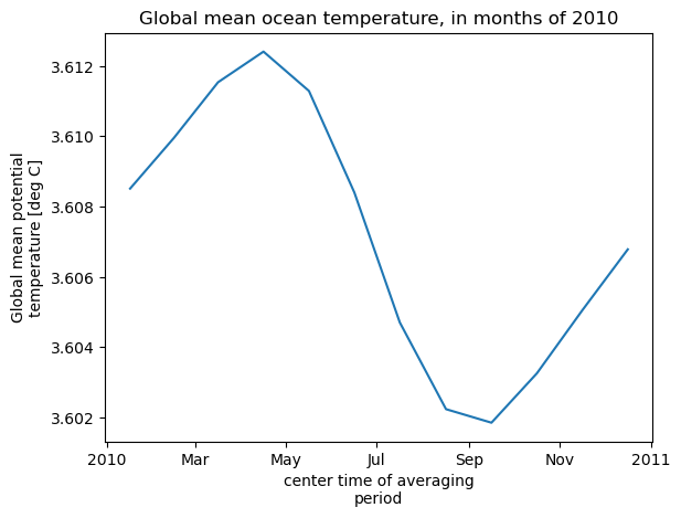
## plot global mean temperature
theta_global_mean = theta_global_mean.assign_attrs(long_name='Global mean potential temperature',units='deg C')
curr_plot = theta_global_mean.plot()
plt.title('Global mean ocean temperature, in months of 2010')
plt.show()

time_log.append(time.time())
time_to_compute = np.diff(np.asarray(time_log)[-2:])[0]

print('\n\nComputation completed')
print(f'Time to open files, 1 process/1 thread: {time_to_open_files} s')
print(f'Time to compute, 1 process/1 thread: {time_to_compute} s')

{'ShortName': 'ECCO_L4_TEMP_SALINITY_LLC0090GRID_MONTHLY_V4R4', 'temporal': '2010-01-02,2010-12-31'}

Total number of matching granules: 12
{'ShortName': 'ECCO_L4_GEOMETRY_LLC0090GRID_V4R4', 'temporal': '1992-01-01,2017-12-31'}

Total number of matching granules: 1

Computation completed
Time to open files, 1 process/1 thread: 35.65613341331482 s
Time to compute, 1 process/1 thread: 9.323273658752441 s
CPU times: user 16.4 s, sys: 4.07 s, total: 20.5 s
Wall time: 45 s

You can see that much more time was spent “opening” the files than actually carrying out the computation. By opening the dataset with optimal chunking, we saved some time on the computations. However, opening files directly from S3 involves some communication between our instance and S3 that is not very efficient.

In the next example, we’ll see if using multiple processes & threads helps speed up this code. But first, let’s have a look at the content of the datasets that we have opened in our workspace:

# dataset with temperature and salinity
ds

<xarray.Dataset> Size: 510MB
Dimensions:    (i: 90, i_g: 90, j: 90, j_g: 90, k: 50, k_u: 50, k_l: 50,
                k_p1: 51, tile: 13, time: 12, nv: 2, nb: 4)
Coordinates: (12/22)
  * i          (i) int32 360B 0 1 2 3 4 5 6 7 8 9 ... 81 82 83 84 85 86 87 88 89
  * i_g        (i_g) int32 360B 0 1 2 3 4 5 6 7 8 ... 81 82 83 84 85 86 87 88 89
  * j          (j) int32 360B 0 1 2 3 4 5 6 7 8 9 ... 81 82 83 84 85 86 87 88 89
  * j_g        (j_g) int32 360B 0 1 2 3 4 5 6 7 8 ... 81 82 83 84 85 86 87 88 89
  * k          (k) int32 200B 0 1 2 3 4 5 6 7 8 9 ... 41 42 43 44 45 46 47 48 49
  * k_u        (k_u) int32 200B 0 1 2 3 4 5 6 7 8 ... 41 42 43 44 45 46 47 48 49
    ...         ...
    Zu         (k_u) float32 200B dask.array<chunksize=(50,), meta=np.ndarray>
    Zl         (k_l) float32 200B dask.array<chunksize=(50,), meta=np.ndarray>
    time_bnds  (time, nv) datetime64[ns] 192B dask.array<chunksize=(1, 2), meta=np.ndarray>
    XC_bnds    (tile, j, i, nb) float32 2MB dask.array<chunksize=(13, 90, 90, 4), meta=np.ndarray>
    YC_bnds    (tile, j, i, nb) float32 2MB dask.array<chunksize=(13, 90, 90, 4), meta=np.ndarray>
    Z_bnds     (k, nv) float32 400B dask.array<chunksize=(10, 2), meta=np.ndarray>
Dimensions without coordinates: nv, nb
Data variables:
    THETA      (time, k, tile, j, i) float32 253MB dask.array<chunksize=(1, 10, 13, 90, 90), meta=np.ndarray>
    SALT       (time, k, tile, j, i) float32 253MB dask.array<chunksize=(1, 10, 13, 90, 90), meta=np.ndarray>
Attributes: (12/62)
    acknowledgement:                 This research was carried out by the Jet...
    author:                          Ian Fenty and Ou Wang
    cdm_data_type:                   Grid
    comment:                         Fields provided on the curvilinear lat-l...
    Conventions:                     CF-1.8, ACDD-1.3
    coordinates_comment:             Note: the global 'coordinates' attribute...
    ...                              ...
    time_coverage_duration:          P1M
    time_coverage_end:               2010-02-01T00:00:00
    time_coverage_resolution:        P1M
    time_coverage_start:             2010-01-01T00:00:00
    title:                           ECCO Ocean Temperature and Salinity - Mo...
    uuid:                            f4291248-4181-11eb-82cd-0cc47a3f446d

xarray.Dataset

• Dimensions:
  • i: 90
  • i_g: 90
  • j: 90
  • j_g: 90
  • k: 50
  • k_u: 50
  • k_l: 50
  • k_p1: 51
  • tile: 13
  • time: 12
  • nv: 2
  • nb: 4
• Coordinates: (22)
  • i
    (i)
    int32
    0 1 2 3 4 5 6 ... 84 85 86 87 88 89

    axis :

    X

    long_name :

    grid index in x for variables at tracer and 'v' locations

    swap_dim :

    XC

    comment :

    In the Arakawa C-grid system, tracer (e.g., THETA) and 'v' variables (e.g., VVEL) have the same x coordinate on the model grid.

    coverage_content_type :

    coordinate

    array([ 0,  1,  2,  3,  4,  5,  6,  7,  8,  9, 10, 11, 12, 13, 14, 15, 16, 17,
           18, 19, 20, 21, 22, 23, 24, 25, 26, 27, 28, 29, 30, 31, 32, 33, 34, 35,
           36, 37, 38, 39, 40, 41, 42, 43, 44, 45, 46, 47, 48, 49, 50, 51, 52, 53,
           54, 55, 56, 57, 58, 59, 60, 61, 62, 63, 64, 65, 66, 67, 68, 69, 70, 71,
           72, 73, 74, 75, 76, 77, 78, 79, 80, 81, 82, 83, 84, 85, 86, 87, 88, 89],
          dtype=int32)

  • i_g
    (i_g)
    int32
    0 1 2 3 4 5 6 ... 84 85 86 87 88 89

    axis :

    X

    long_name :

    grid index in x for variables at 'u' and 'g' locations

    c_grid_axis_shift :

    -0.5

    swap_dim :

    XG

    comment :

    In the Arakawa C-grid system, 'u' (e.g., UVEL) and 'g' variables (e.g., XG) have the same x coordinate on the model grid.

    coverage_content_type :

    coordinate

    array([ 0,  1,  2,  3,  4,  5,  6,  7,  8,  9, 10, 11, 12, 13, 14, 15, 16, 17,
           18, 19, 20, 21, 22, 23, 24, 25, 26, 27, 28, 29, 30, 31, 32, 33, 34, 35,
           36, 37, 38, 39, 40, 41, 42, 43, 44, 45, 46, 47, 48, 49, 50, 51, 52, 53,
           54, 55, 56, 57, 58, 59, 60, 61, 62, 63, 64, 65, 66, 67, 68, 69, 70, 71,
           72, 73, 74, 75, 76, 77, 78, 79, 80, 81, 82, 83, 84, 85, 86, 87, 88, 89],
          dtype=int32)

  • j
    (j)
    int32
    0 1 2 3 4 5 6 ... 84 85 86 87 88 89

    axis :

    Y

    long_name :

    grid index in y for variables at tracer and 'u' locations

    swap_dim :

    YC

    comment :

    In the Arakawa C-grid system, tracer (e.g., THETA) and 'u' variables (e.g., UVEL) have the same y coordinate on the model grid.

    coverage_content_type :

    coordinate

    array([ 0,  1,  2,  3,  4,  5,  6,  7,  8,  9, 10, 11, 12, 13, 14, 15, 16, 17,
           18, 19, 20, 21, 22, 23, 24, 25, 26, 27, 28, 29, 30, 31, 32, 33, 34, 35,
           36, 37, 38, 39, 40, 41, 42, 43, 44, 45, 46, 47, 48, 49, 50, 51, 52, 53,
           54, 55, 56, 57, 58, 59, 60, 61, 62, 63, 64, 65, 66, 67, 68, 69, 70, 71,
           72, 73, 74, 75, 76, 77, 78, 79, 80, 81, 82, 83, 84, 85, 86, 87, 88, 89],
          dtype=int32)

  • j_g
    (j_g)
    int32
    0 1 2 3 4 5 6 ... 84 85 86 87 88 89

    axis :

    Y

    long_name :

    grid index in y for variables at 'v' and 'g' locations

    c_grid_axis_shift :

    -0.5

    swap_dim :

    YG

    comment :

    In the Arakawa C-grid system, 'v' (e.g., VVEL) and 'g' variables (e.g., XG) have the same y coordinate.

    coverage_content_type :

    coordinate

    array([ 0,  1,  2,  3,  4,  5,  6,  7,  8,  9, 10, 11, 12, 13, 14, 15, 16, 17,
           18, 19, 20, 21, 22, 23, 24, 25, 26, 27, 28, 29, 30, 31, 32, 33, 34, 35,
           36, 37, 38, 39, 40, 41, 42, 43, 44, 45, 46, 47, 48, 49, 50, 51, 52, 53,
           54, 55, 56, 57, 58, 59, 60, 61, 62, 63, 64, 65, 66, 67, 68, 69, 70, 71,
           72, 73, 74, 75, 76, 77, 78, 79, 80, 81, 82, 83, 84, 85, 86, 87, 88, 89],
          dtype=int32)

  • k
    (k)
    int32
    0 1 2 3 4 5 6 ... 44 45 46 47 48 49

    axis :

    Z

    long_name :

    grid index in z for tracer variables

    swap_dim :

    Z

    coverage_content_type :

    coordinate

    array([ 0,  1,  2,  3,  4,  5,  6,  7,  8,  9, 10, 11, 12, 13, 14, 15, 16, 17,
           18, 19, 20, 21, 22, 23, 24, 25, 26, 27, 28, 29, 30, 31, 32, 33, 34, 35,
           36, 37, 38, 39, 40, 41, 42, 43, 44, 45, 46, 47, 48, 49], dtype=int32)

  • k_u
    (k_u)
    int32
    0 1 2 3 4 5 6 ... 44 45 46 47 48 49

    axis :

    Z

    c_grid_axis_shift :

    0.5

    swap_dim :

    Zu

    coverage_content_type :

    coordinate

    long_name :

    grid index in z corresponding to the bottom face of tracer grid cells ('w' locations)

    comment :

    First index corresponds to the bottom surface of the uppermost tracer grid cell. The use of 'u' in the variable name follows the MITgcm convention for ocean variables in which the upper (u) face of a tracer grid cell on the logical grid corresponds to the bottom face of the grid cell on the physical grid.

    array([ 0,  1,  2,  3,  4,  5,  6,  7,  8,  9, 10, 11, 12, 13, 14, 15, 16, 17,
           18, 19, 20, 21, 22, 23, 24, 25, 26, 27, 28, 29, 30, 31, 32, 33, 34, 35,
           36, 37, 38, 39, 40, 41, 42, 43, 44, 45, 46, 47, 48, 49], dtype=int32)

  • k_l
    (k_l)
    int32
    0 1 2 3 4 5 6 ... 44 45 46 47 48 49

    axis :

    Z

    c_grid_axis_shift :

    -0.5

    swap_dim :

    Zl

    coverage_content_type :

    coordinate

    long_name :

    grid index in z corresponding to the top face of tracer grid cells ('w' locations)

    comment :

    First index corresponds to the top surface of the uppermost tracer grid cell. The use of 'l' in the variable name follows the MITgcm convention for ocean variables in which the lower (l) face of a tracer grid cell on the logical grid corresponds to the top face of the grid cell on the physical grid.

    array([ 0,  1,  2,  3,  4,  5,  6,  7,  8,  9, 10, 11, 12, 13, 14, 15, 16, 17,
           18, 19, 20, 21, 22, 23, 24, 25, 26, 27, 28, 29, 30, 31, 32, 33, 34, 35,
           36, 37, 38, 39, 40, 41, 42, 43, 44, 45, 46, 47, 48, 49], dtype=int32)

  • k_p1
    (k_p1)
    int32
    0 1 2 3 4 5 6 ... 45 46 47 48 49 50

    axis :

    Z

    long_name :

    grid index in z for variables at 'w' locations

    c_grid_axis_shift :

    [-0.5 0.5]

    swap_dim :

    Zp1

    comment :

    Includes top of uppermost model tracer cell (k_p1=0) and bottom of lowermost tracer cell (k_p1=51).

    coverage_content_type :

    coordinate

    array([ 0,  1,  2,  3,  4,  5,  6,  7,  8,  9, 10, 11, 12, 13, 14, 15, 16, 17,
           18, 19, 20, 21, 22, 23, 24, 25, 26, 27, 28, 29, 30, 31, 32, 33, 34, 35,
           36, 37, 38, 39, 40, 41, 42, 43, 44, 45, 46, 47, 48, 49, 50], dtype=int32)

  • tile
    (tile)
    int32
    0 1 2 3 4 5 6 7 8 9 10 11 12

    long_name :

    lat-lon-cap tile index

    comment :

    The ECCO V4 horizontal model grid is divided into 13 tiles of 90x90 cells for convenience.

    coverage_content_type :

    coordinate

    array([ 0,  1,  2,  3,  4,  5,  6,  7,  8,  9, 10, 11, 12], dtype=int32)

  • time
    (time)
    datetime64[ns]
    2010-01-16T12:00:00 ... 2010-12-...

    long_name :

    center time of averaging period

    axis :

    T

    bounds :

    time_bnds

    coverage_content_type :

    coordinate

    standard_name :

    time

    array(['2010-01-16T12:00:00.000000000', '2010-02-15T00:00:00.000000000',
           '2010-03-16T12:00:00.000000000', '2010-04-16T00:00:00.000000000',
           '2010-05-16T12:00:00.000000000', '2010-06-16T00:00:00.000000000',
           '2010-07-16T12:00:00.000000000', '2010-08-16T12:00:00.000000000',
           '2010-09-16T00:00:00.000000000', '2010-10-16T12:00:00.000000000',
           '2010-11-16T00:00:00.000000000', '2010-12-16T12:00:00.000000000'],
          dtype='datetime64[ns]')

  • XC
    (tile, j, i)
    float32
    dask.array<chunksize=(13, 90, 90), meta=np.ndarray>

    long_name :

    longitude of tracer grid cell center

    units :

    degrees_east

    coordinate :

    YC XC

    bounds :

    XC_bnds

    comment :

    nonuniform grid spacing

    coverage_content_type :

    coordinate

    standard_name :

    longitude

    Array Chunk Bytes 411.33 kiB 411.33 kiB Shape (13, 90, 90) (13, 90, 90) Dask graph 1 chunks in 2 graph layers Data type float32 numpy.ndarray

  • YC
    (tile, j, i)
    float32
    dask.array<chunksize=(13, 90, 90), meta=np.ndarray>

    long_name :

    latitude of tracer grid cell center

    units :

    degrees_north

    coordinate :

    YC XC

    bounds :

    YC_bnds

    comment :

    nonuniform grid spacing

    coverage_content_type :

    coordinate

    standard_name :

    latitude

    Array Chunk Bytes 411.33 kiB 411.33 kiB Shape (13, 90, 90) (13, 90, 90) Dask graph 1 chunks in 2 graph layers Data type float32 numpy.ndarray

  • XG
    (tile, j_g, i_g)
    float32
    dask.array<chunksize=(13, 90, 90), meta=np.ndarray>

    long_name :

    longitude of 'southwest' corner of tracer grid cell

    units :

    degrees_east

    coordinate :

    YG XG

    comment :

    Nonuniform grid spacing. Note: 'southwest' does not correspond to geographic orientation but is used for convenience to describe the computational grid. See MITgcm dcoumentation for details.

    coverage_content_type :

    coordinate

    standard_name :

    longitude

    Array Chunk Bytes 411.33 kiB 411.33 kiB Shape (13, 90, 90) (13, 90, 90) Dask graph 1 chunks in 2 graph layers Data type float32 numpy.ndarray

  • YG
    (tile, j_g, i_g)
    float32
    dask.array<chunksize=(13, 90, 90), meta=np.ndarray>

    long_name :

    latitude of 'southwest' corner of tracer grid cell

    units :

    degrees_north

    coordinate :

    YG XG

    comment :

    Nonuniform grid spacing. Note: 'southwest' does not correspond to geographic orientation but is used for convenience to describe the computational grid. See MITgcm dcoumentation for details.

    coverage_content_type :

    coordinate

    standard_name :

    latitude

    Array Chunk Bytes 411.33 kiB 411.33 kiB Shape (13, 90, 90) (13, 90, 90) Dask graph 1 chunks in 2 graph layers Data type float32 numpy.ndarray

  • Z
    (k)
    float32
    dask.array<chunksize=(10,), meta=np.ndarray>

    long_name :

    depth of tracer grid cell center

    units :

    m

    positive :

    up

    bounds :

    Z_bnds

    comment :

    Non-uniform vertical spacing.

    coverage_content_type :

    coordinate

    standard_name :

    depth

    Array Chunk Bytes 200 B 40 B Shape (50,) (10,) Dask graph 5 chunks in 2 graph layers Data type float32 numpy.ndarray

  • Zp1
    (k_p1)
    float32
    dask.array<chunksize=(51,), meta=np.ndarray>

    long_name :

    depth of tracer grid cell interface

    units :

    m

    positive :

    up

    comment :

    Contains one element more than the number of vertical layers. First element is 0m, the depth of the upper interface of the surface grid cell. Last element is the depth of the lower interface of the deepest grid cell.

    coverage_content_type :

    coordinate

    standard_name :

    depth

    Array Chunk Bytes 204 B 204 B Shape (51,) (51,) Dask graph 1 chunks in 2 graph layers Data type float32 numpy.ndarray

  • Zu
    (k_u)
    float32
    dask.array<chunksize=(50,), meta=np.ndarray>

    units :

    m

    positive :

    up

    coverage_content_type :

    coordinate

    standard_name :

    depth

    long_name :

    depth of the bottom face of tracer grid cells

    comment :

    First element is -10m, the depth of the bottom face of the first tracer grid cell. Last element is the depth of the bottom face of the deepest grid cell. The use of 'u' in the variable name follows the MITgcm convention for ocean variables in which the upper (u) face of a tracer grid cell on the logical grid corresponds to the bottom face of the grid cell on the physical grid. In other words, the logical vertical grid of MITgcm ocean variables is inverted relative to the physical vertical grid.

    Array Chunk Bytes 200 B 200 B Shape (50,) (50,) Dask graph 1 chunks in 2 graph layers Data type float32 numpy.ndarray

  • Zl
    (k_l)
    float32
    dask.array<chunksize=(50,), meta=np.ndarray>

    units :

    m

    positive :

    up

    coverage_content_type :

    coordinate

    standard_name :

    depth

    long_name :

    depth of the top face of tracer grid cells

    comment :

    First element is 0m, the depth of the top face of the first tracer grid cell (ocean surface). Last element is the depth of the top face of the deepest grid cell. The use of 'l' in the variable name follows the MITgcm convention for ocean variables in which the lower (l) face of a tracer grid cell on the logical grid corresponds to the top face of the grid cell on the physical grid. In other words, the logical vertical grid of MITgcm ocean variables is inverted relative to the physical vertical grid.

    Array Chunk Bytes 200 B 200 B Shape (50,) (50,) Dask graph 1 chunks in 2 graph layers Data type float32 numpy.ndarray

  • time_bnds
    (time, nv)
    datetime64[ns]
    dask.array<chunksize=(1, 2), meta=np.ndarray>

    comment :

    Start and end times of averaging period.

    coverage_content_type :

    coordinate

    long_name :

    time bounds of averaging period

    Array Chunk Bytes 192 B 16 B Shape (12, 2) (1, 2) Dask graph 12 chunks in 25 graph layers Data type datetime64[ns] numpy.ndarray

  • XC_bnds
    (tile, j, i, nb)
    float32
    dask.array<chunksize=(13, 90, 90, 4), meta=np.ndarray>

    comment :

    Bounds array follows CF conventions. XC_bnds[i,j,0] = 'southwest' corner (j-1, i-1), XC_bnds[i,j,1] = 'southeast' corner (j-1, i+1), XC_bnds[i,j,2] = 'northeast' corner (j+1, i+1), XC_bnds[i,j,3] = 'northwest' corner (j+1, i-1). Note: 'southwest', 'southeast', northwest', and 'northeast' do not correspond to geographic orientation but are used for convenience to describe the computational grid. See MITgcm dcoumentation for details.

    coverage_content_type :

    coordinate

    long_name :

    longitudes of tracer grid cell corners

    Array Chunk Bytes 1.61 MiB 1.61 MiB Shape (13, 90, 90, 4) (13, 90, 90, 4) Dask graph 1 chunks in 2 graph layers Data type float32 numpy.ndarray

  • YC_bnds
    (tile, j, i, nb)
    float32
    dask.array<chunksize=(13, 90, 90, 4), meta=np.ndarray>

    comment :

    Bounds array follows CF conventions. YC_bnds[i,j,0] = 'southwest' corner (j-1, i-1), YC_bnds[i,j,1] = 'southeast' corner (j-1, i+1), YC_bnds[i,j,2] = 'northeast' corner (j+1, i+1), YC_bnds[i,j,3] = 'northwest' corner (j+1, i-1). Note: 'southwest', 'southeast', northwest', and 'northeast' do not correspond to geographic orientation but are used for convenience to describe the computational grid. See MITgcm dcoumentation for details.

    coverage_content_type :

    coordinate

    long_name :

    latitudes of tracer grid cell corners

    Array Chunk Bytes 1.61 MiB 1.61 MiB Shape (13, 90, 90, 4) (13, 90, 90, 4) Dask graph 1 chunks in 2 graph layers Data type float32 numpy.ndarray

  • Z_bnds
    (k, nv)
    float32
    dask.array<chunksize=(10, 2), meta=np.ndarray>

    comment :

    One pair of depths for each vertical level.

    coverage_content_type :

    coordinate

    long_name :

    depths of tracer grid cell upper and lower interfaces

    Array Chunk Bytes 400 B 80 B Shape (50, 2) (10, 2) Dask graph 5 chunks in 2 graph layers Data type float32 numpy.ndarray

• Data variables: (2)
  • THETA
    (time, k, tile, j, i)
    float32
    dask.array<chunksize=(1, 10, 13, 90, 90), meta=np.ndarray>

    long_name :

    Potential temperature

    units :

    degree_C

    coverage_content_type :

    modelResult

    standard_name :

    sea_water_potential_temperature

    comment :

    Sea water potential temperature is the temperature a parcel of sea water would have if moved adiabatically to sea level pressure. Note: the equation of state is a modified UNESCO formula by Jackett and McDougall (1995), which uses the model variable potential temperature as input assuming a horizontally and temporally constant pressure of $p_0=-g \rho_{0} z$.

    valid_min :

    -2.2909388542175293

    valid_max :

    36.032955169677734

    Array Chunk Bytes 241.01 MiB 4.02 MiB Shape (12, 50, 13, 90, 90) (1, 10, 13, 90, 90) Dask graph 60 chunks in 25 graph layers Data type float32 numpy.ndarray

  • SALT
    (time, k, tile, j, i)
    float32
    dask.array<chunksize=(1, 10, 13, 90, 90), meta=np.ndarray>

    long_name :

    Salinity

    units :

    1e-3

    coverage_content_type :

    modelResult

    standard_name :

    sea_water_salinity

    valid_min :

    17.106637954711914

    valid_max :

    41.26802444458008

    comment :

    Defined using CF convention 'Sea water salinity is the salt content of sea water, often on the Practical Salinity Scale of 1978. However, the unqualified term 'salinity' is generic and does not necessarily imply any particular method of calculation. The units of salinity are dimensionless and the units attribute should normally be given as 1e-3 or 0.001 i.e. parts per thousand.' see https://cfconventions.org/Data/cf-standard-names/73/build/cf-standard-name-table.html

    Array Chunk Bytes 241.01 MiB 4.02 MiB Shape (12, 50, 13, 90, 90) (1, 10, 13, 90, 90) Dask graph 60 chunks in 25 graph layers Data type float32 numpy.ndarray

• Indexes: (10)
  • i
    PandasIndex

    PandasIndex(Index([ 0,  1,  2,  3,  4,  5,  6,  7,  8,  9, 10, 11, 12, 13, 14, 15, 16, 17,
           18, 19, 20, 21, 22, 23, 24, 25, 26, 27, 28, 29, 30, 31, 32, 33, 34, 35,
           36, 37, 38, 39, 40, 41, 42, 43, 44, 45, 46, 47, 48, 49, 50, 51, 52, 53,
           54, 55, 56, 57, 58, 59, 60, 61, 62, 63, 64, 65, 66, 67, 68, 69, 70, 71,
           72, 73, 74, 75, 76, 77, 78, 79, 80, 81, 82, 83, 84, 85, 86, 87, 88, 89],
          dtype='int32', name='i'))

  • i_g
    PandasIndex

    PandasIndex(Index([ 0,  1,  2,  3,  4,  5,  6,  7,  8,  9, 10, 11, 12, 13, 14, 15, 16, 17,
           18, 19, 20, 21, 22, 23, 24, 25, 26, 27, 28, 29, 30, 31, 32, 33, 34, 35,
           36, 37, 38, 39, 40, 41, 42, 43, 44, 45, 46, 47, 48, 49, 50, 51, 52, 53,
           54, 55, 56, 57, 58, 59, 60, 61, 62, 63, 64, 65, 66, 67, 68, 69, 70, 71,
           72, 73, 74, 75, 76, 77, 78, 79, 80, 81, 82, 83, 84, 85, 86, 87, 88, 89],
          dtype='int32', name='i_g'))

  • j
    PandasIndex

    PandasIndex(Index([ 0,  1,  2,  3,  4,  5,  6,  7,  8,  9, 10, 11, 12, 13, 14, 15, 16, 17,
           18, 19, 20, 21, 22, 23, 24, 25, 26, 27, 28, 29, 30, 31, 32, 33, 34, 35,
           36, 37, 38, 39, 40, 41, 42, 43, 44, 45, 46, 47, 48, 49, 50, 51, 52, 53,
           54, 55, 56, 57, 58, 59, 60, 61, 62, 63, 64, 65, 66, 67, 68, 69, 70, 71,
           72, 73, 74, 75, 76, 77, 78, 79, 80, 81, 82, 83, 84, 85, 86, 87, 88, 89],
          dtype='int32', name='j'))

  • j_g
    PandasIndex

    PandasIndex(Index([ 0,  1,  2,  3,  4,  5,  6,  7,  8,  9, 10, 11, 12, 13, 14, 15, 16, 17,
           18, 19, 20, 21, 22, 23, 24, 25, 26, 27, 28, 29, 30, 31, 32, 33, 34, 35,
           36, 37, 38, 39, 40, 41, 42, 43, 44, 45, 46, 47, 48, 49, 50, 51, 52, 53,
           54, 55, 56, 57, 58, 59, 60, 61, 62, 63, 64, 65, 66, 67, 68, 69, 70, 71,
           72, 73, 74, 75, 76, 77, 78, 79, 80, 81, 82, 83, 84, 85, 86, 87, 88, 89],
          dtype='int32', name='j_g'))

  • k
    PandasIndex

    PandasIndex(Index([ 0,  1,  2,  3,  4,  5,  6,  7,  8,  9, 10, 11, 12, 13, 14, 15, 16, 17,
           18, 19, 20, 21, 22, 23, 24, 25, 26, 27, 28, 29, 30, 31, 32, 33, 34, 35,
           36, 37, 38, 39, 40, 41, 42, 43, 44, 45, 46, 47, 48, 49],
          dtype='int32', name='k'))

  • k_u
    PandasIndex

    PandasIndex(Index([ 0,  1,  2,  3,  4,  5,  6,  7,  8,  9, 10, 11, 12, 13, 14, 15, 16, 17,
           18, 19, 20, 21, 22, 23, 24, 25, 26, 27, 28, 29, 30, 31, 32, 33, 34, 35,
           36, 37, 38, 39, 40, 41, 42, 43, 44, 45, 46, 47, 48, 49],
          dtype='int32', name='k_u'))

  • k_l
    PandasIndex

    PandasIndex(Index([ 0,  1,  2,  3,  4,  5,  6,  7,  8,  9, 10, 11, 12, 13, 14, 15, 16, 17,
           18, 19, 20, 21, 22, 23, 24, 25, 26, 27, 28, 29, 30, 31, 32, 33, 34, 35,
           36, 37, 38, 39, 40, 41, 42, 43, 44, 45, 46, 47, 48, 49],
          dtype='int32', name='k_l'))

  • k_p1
    PandasIndex

    PandasIndex(Index([ 0,  1,  2,  3,  4,  5,  6,  7,  8,  9, 10, 11, 12, 13, 14, 15, 16, 17,
           18, 19, 20, 21, 22, 23, 24, 25, 26, 27, 28, 29, 30, 31, 32, 33, 34, 35,
           36, 37, 38, 39, 40, 41, 42, 43, 44, 45, 46, 47, 48, 49, 50],
          dtype='int32', name='k_p1'))

  • tile
    PandasIndex

    PandasIndex(Index([0, 1, 2, 3, 4, 5, 6, 7, 8, 9, 10, 11, 12], dtype='int32', name='tile'))

  • time
    PandasIndex

    PandasIndex(DatetimeIndex(['2010-01-16 12:00:00', '2010-02-15 00:00:00',
                   '2010-03-16 12:00:00', '2010-04-16 00:00:00',
                   '2010-05-16 12:00:00', '2010-06-16 00:00:00',
                   '2010-07-16 12:00:00', '2010-08-16 12:00:00',
                   '2010-09-16 00:00:00', '2010-10-16 12:00:00',
                   '2010-11-16 00:00:00', '2010-12-16 12:00:00'],
                  dtype='datetime64[ns]', name='time', freq=None))

• Attributes: (62)

  acknowledgement :

  This research was carried out by the Jet Propulsion Laboratory, managed by the California Institute of Technology under a contract with the National Aeronautics and Space Administration.

  author :

  Ian Fenty and Ou Wang

  cdm_data_type :

  Grid

  comment :

  Fields provided on the curvilinear lat-lon-cap 90 (llc90) native grid used in the ECCO model.

  Conventions :

  CF-1.8, ACDD-1.3

  coordinates_comment :

  Note: the global 'coordinates' attribute describes auxillary coordinates.

  creator_email :

  ecco-group@mit.edu

  creator_institution :

  NASA Jet Propulsion Laboratory (JPL)

  creator_name :

  ECCO Consortium

  creator_type :

  group

  creator_url :

  https://ecco-group.org

  date_created :

  2020-12-18T14:39:56

  date_issued :

  2020-12-18T14:39:56

  date_metadata_modified :

  2021-03-15T21:55:41

  date_modified :

  2021-03-15T21:55:41

  geospatial_bounds_crs :

  EPSG:4326

  geospatial_lat_max :

  90.0

  geospatial_lat_min :

  -90.0

  geospatial_lat_resolution :

  variable

  geospatial_lat_units :

  degrees_north

  geospatial_lon_max :

  180.0

  geospatial_lon_min :

  -180.0

  geospatial_lon_resolution :

  variable

  geospatial_lon_units :

  degrees_east

  geospatial_vertical_max :

  0.0

  geospatial_vertical_min :

  -6134.5

  geospatial_vertical_positive :

  up

  geospatial_vertical_resolution :

  variable

  geospatial_vertical_units :

  meter

  history :

  Inaugural release of an ECCO Central Estimate solution to PO.DAAC

  id :

  10.5067/ECL5M-OTS44

  institution :

  NASA Jet Propulsion Laboratory (JPL)

  instrument_vocabulary :

  GCMD instrument keywords

  keywords :

  EARTH SCIENCE > OCEANS > OCEAN TEMPERATURE > POTENTIAL TEMPERATURE, EARTH SCIENCE > OCEANS > SALINITY/DENSITY > SALINITY, EARTH SCIENCE SERVICES > MODELS > EARTH SCIENCE REANALYSES/ASSIMILATION MODELS

  keywords_vocabulary :

  NASA Global Change Master Directory (GCMD) Science Keywords

  license :

  Public Domain

  metadata_link :

  https://cmr.earthdata.nasa.gov/search/collections.umm_json?ShortName=ECCO_L4_TEMP_SALINITY_LLC0090GRID_MONTHLY_V4R4

  naming_authority :

  gov.nasa.jpl

  platform :

  ERS-1/2, TOPEX/Poseidon, Geosat Follow-On (GFO), ENVISAT, Jason-1, Jason-2, CryoSat-2, SARAL/AltiKa, Jason-3, AVHRR, Aquarius, SSM/I, SSMIS, GRACE, DTU17MDT, Argo, WOCE, GO-SHIP, MEOP, Ice Tethered Profilers (ITP)

  platform_vocabulary :

  GCMD platform keywords

  processing_level :

  L4

  product_name :

  OCEAN_TEMPERATURE_SALINITY_mon_mean_2010-01_ECCO_V4r4_native_llc0090.nc

  product_time_coverage_end :

  2018-01-01T00:00:00

  product_time_coverage_start :

  1992-01-01T12:00:00

  product_version :

  Version 4, Release 4

  program :

  NASA Physical Oceanography, Cryosphere, Modeling, Analysis, and Prediction (MAP)

  project :

  Estimating the Circulation and Climate of the Ocean (ECCO)

  publisher_email :

  podaac@podaac.jpl.nasa.gov

  publisher_institution :

  PO.DAAC

  publisher_name :

  Physical Oceanography Distributed Active Archive Center (PO.DAAC)

  publisher_type :

  institution

  publisher_url :

  https://podaac.jpl.nasa.gov

  references :

  ECCO Consortium, Fukumori, I., Wang, O., Fenty, I., Forget, G., Heimbach, P., & Ponte, R. M. 2020. Synopsis of the ECCO Central Production Global Ocean and Sea-Ice State Estimate (Version 4 Release 4). doi:10.5281/zenodo.3765928

  source :

  The ECCO V4r4 state estimate was produced by fitting a free-running solution of the MITgcm (checkpoint 66g) to satellite and in situ observational data in a least squares sense using the adjoint method

  standard_name_vocabulary :

  NetCDF Climate and Forecast (CF) Metadata Convention

  summary :

  This dataset provides monthly-averaged ocean potential temperature and salinity on the lat-lon-cap 90 (llc90) native model grid from the ECCO Version 4 Release 4 (V4r4) ocean and sea-ice state estimate. Estimating the Circulation and Climate of the Ocean (ECCO) state estimates are dynamically and kinematically-consistent reconstructions of the three-dimensional, time-evolving ocean, sea-ice, and surface atmospheric states. ECCO V4r4 is a free-running solution of a global, nominally 1-degree configuration of the MIT general circulation model (MITgcm) that has been fit to observations in a least-squares sense. Observational data constraints used in V4r4 include sea surface height (SSH) from satellite altimeters [ERS-1/2, TOPEX/Poseidon, GFO, ENVISAT, Jason-1,2,3, CryoSat-2, and SARAL/AltiKa]; sea surface temperature (SST) from satellite radiometers [AVHRR], sea surface salinity (SSS) from the Aquarius satellite radiometer/scatterometer, ocean bottom pressure (OBP) from the GRACE satellite gravimeter; sea-ice concentration from satellite radiometers [SSM/I and SSMIS], and in-situ ocean temperature and salinity measured with conductivity-temperature-depth (CTD) sensors and expendable bathythermographs (XBTs) from several programs [e.g., WOCE, GO-SHIP, Argo, and others] and platforms [e.g., research vessels, gliders, moorings, ice-tethered profilers, and instrumented pinnipeds]. V4r4 covers the period 1992-01-01T12:00:00 to 2018-01-01T00:00:00.

  time_coverage_duration :

  P1M

  time_coverage_end :

  2010-02-01T00:00:00

  time_coverage_resolution :

  P1M

  time_coverage_start :

  2010-01-01T00:00:00

  title :

  ECCO Ocean Temperature and Salinity - Monthly Mean llc90 Grid (Version 4 Release 4)

  uuid :

  f4291248-4181-11eb-82cd-0cc47a3f446d

# grid parameters dataset
ds_grid

<xarray.Dataset> Size: 89MB
Dimensions:  (i: 90, i_g: 90, j: 90, j_g: 90, k: 50, k_u: 50, k_l: 50,
              k_p1: 51, tile: 13, nb: 4, nv: 2)
Coordinates: (12/20)
  * i        (i) int32 360B 0 1 2 3 4 5 6 7 8 9 ... 81 82 83 84 85 86 87 88 89
  * i_g      (i_g) int32 360B 0 1 2 3 4 5 6 7 8 9 ... 81 82 83 84 85 86 87 88 89
  * j        (j) int32 360B 0 1 2 3 4 5 6 7 8 9 ... 81 82 83 84 85 86 87 88 89
  * j_g      (j_g) int32 360B 0 1 2 3 4 5 6 7 8 9 ... 81 82 83 84 85 86 87 88 89
  * k        (k) int32 200B 0 1 2 3 4 5 6 7 8 9 ... 41 42 43 44 45 46 47 48 49
  * k_u      (k_u) int32 200B 0 1 2 3 4 5 6 7 8 9 ... 41 42 43 44 45 46 47 48 49
    ...       ...
    Zp1      (k_p1) float32 204B dask.array<chunksize=(51,), meta=np.ndarray>
    Zu       (k_u) float32 200B dask.array<chunksize=(50,), meta=np.ndarray>
    Zl       (k_l) float32 200B dask.array<chunksize=(50,), meta=np.ndarray>
    XC_bnds  (tile, j, i, nb) float32 2MB dask.array<chunksize=(13, 90, 90, 4), meta=np.ndarray>
    YC_bnds  (tile, j, i, nb) float32 2MB dask.array<chunksize=(13, 90, 90, 4), meta=np.ndarray>
    Z_bnds   (k, nv) float32 400B dask.array<chunksize=(10, 2), meta=np.ndarray>
Dimensions without coordinates: nb, nv
Data variables: (12/21)
    CS       (tile, j, i) float32 421kB dask.array<chunksize=(13, 90, 90), meta=np.ndarray>
    SN       (tile, j, i) float32 421kB dask.array<chunksize=(13, 90, 90), meta=np.ndarray>
    rA       (tile, j, i) float32 421kB dask.array<chunksize=(13, 90, 90), meta=np.ndarray>
    dxG      (tile, j_g, i) float32 421kB dask.array<chunksize=(13, 90, 90), meta=np.ndarray>
    dyG      (tile, j, i_g) float32 421kB dask.array<chunksize=(13, 90, 90), meta=np.ndarray>
    Depth    (tile, j, i) float32 421kB dask.array<chunksize=(13, 90, 90), meta=np.ndarray>
    ...       ...
    hFacC    (k, tile, j, i) float32 21MB dask.array<chunksize=(10, 13, 90, 90), meta=np.ndarray>
    hFacW    (k, tile, j, i_g) float32 21MB dask.array<chunksize=(10, 13, 90, 45), meta=np.ndarray>
    hFacS    (k, tile, j_g, i) float32 21MB dask.array<chunksize=(10, 13, 45, 90), meta=np.ndarray>
    maskC    (k, tile, j, i) bool 5MB dask.array<chunksize=(10, 13, 90, 90), meta=np.ndarray>
    maskW    (k, tile, j, i_g) bool 5MB dask.array<chunksize=(10, 13, 90, 45), meta=np.ndarray>
    maskS    (k, tile, j_g, i) bool 5MB dask.array<chunksize=(10, 13, 45, 90), meta=np.ndarray>
Attributes: (12/58)
    acknowledgement:                 This research was carried out by the Jet...
    author:                          Ian Fenty and Ou Wang
    cdm_data_type:                   Grid
    comment:                         Fields provided on the curvilinear lat-l...
    Conventions:                     CF-1.8, ACDD-1.3
    coordinates_comment:             Note: the global 'coordinates' attribute...
    ...                              ...
    references:                      ECCO Consortium, Fukumori, I., Wang, O.,...
    source:                          The ECCO V4r4 state estimate was produce...
    standard_name_vocabulary:        NetCDF Climate and Forecast (CF) Metadat...
    summary:                         This dataset provides geometric paramete...
    title:                           ECCO Geometry Parameters for the Lat-Lon...
    uuid:                            87ff7d24-86e5-11eb-9c5f-f8f21e2ee3e0

xarray.Dataset

• Dimensions:
  • i: 90
  • i_g: 90
  • j: 90
  • j_g: 90
  • k: 50
  • k_u: 50
  • k_l: 50
  • k_p1: 51
  • tile: 13
  • nb: 4
  • nv: 2
• Coordinates: (20)
  • i
    (i)
    int32
    0 1 2 3 4 5 6 ... 84 85 86 87 88 89

    axis :

    X

    long_name :

    grid index in x for variables at tracer and 'v' locations

    swap_dim :

    XC

    comment :

    In the Arakawa C-grid system, tracer (e.g., THETA) and 'v' variables (e.g., VVEL) have the same x coordinate on the model grid.

    coverage_content_type :

    coordinate

    array([ 0,  1,  2,  3,  4,  5,  6,  7,  8,  9, 10, 11, 12, 13, 14, 15, 16, 17,
           18, 19, 20, 21, 22, 23, 24, 25, 26, 27, 28, 29, 30, 31, 32, 33, 34, 35,
           36, 37, 38, 39, 40, 41, 42, 43, 44, 45, 46, 47, 48, 49, 50, 51, 52, 53,
           54, 55, 56, 57, 58, 59, 60, 61, 62, 63, 64, 65, 66, 67, 68, 69, 70, 71,
           72, 73, 74, 75, 76, 77, 78, 79, 80, 81, 82, 83, 84, 85, 86, 87, 88, 89],
          dtype=int32)

  • i_g
    (i_g)
    int32
    0 1 2 3 4 5 6 ... 84 85 86 87 88 89

    axis :

    X

    long_name :

    grid index in x for variables at 'u' and 'g' locations

    c_grid_axis_shift :

    -0.5

    swap_dim :

    XG

    comment :

    In the Arakawa C-grid system, 'u' (e.g., UVEL) and 'g' variables (e.g., XG) have the same x coordinate on the model grid.

    coverage_content_type :

    coordinate

    array([ 0,  1,  2,  3,  4,  5,  6,  7,  8,  9, 10, 11, 12, 13, 14, 15, 16, 17,
           18, 19, 20, 21, 22, 23, 24, 25, 26, 27, 28, 29, 30, 31, 32, 33, 34, 35,
           36, 37, 38, 39, 40, 41, 42, 43, 44, 45, 46, 47, 48, 49, 50, 51, 52, 53,
           54, 55, 56, 57, 58, 59, 60, 61, 62, 63, 64, 65, 66, 67, 68, 69, 70, 71,
           72, 73, 74, 75, 76, 77, 78, 79, 80, 81, 82, 83, 84, 85, 86, 87, 88, 89],
          dtype=int32)

  • j
    (j)
    int32
    0 1 2 3 4 5 6 ... 84 85 86 87 88 89

    axis :

    Y

    long_name :

    grid index in y for variables at tracer and 'u' locations

    swap_dim :

    YC

    comment :

    In the Arakawa C-grid system, tracer (e.g., THETA) and 'u' variables (e.g., UVEL) have the same y coordinate on the model grid.

    coverage_content_type :

    coordinate

    array([ 0,  1,  2,  3,  4,  5,  6,  7,  8,  9, 10, 11, 12, 13, 14, 15, 16, 17,
           18, 19, 20, 21, 22, 23, 24, 25, 26, 27, 28, 29, 30, 31, 32, 33, 34, 35,
           36, 37, 38, 39, 40, 41, 42, 43, 44, 45, 46, 47, 48, 49, 50, 51, 52, 53,
           54, 55, 56, 57, 58, 59, 60, 61, 62, 63, 64, 65, 66, 67, 68, 69, 70, 71,
           72, 73, 74, 75, 76, 77, 78, 79, 80, 81, 82, 83, 84, 85, 86, 87, 88, 89],
          dtype=int32)

  • j_g
    (j_g)
    int32
    0 1 2 3 4 5 6 ... 84 85 86 87 88 89

    axis :

    Y

    long_name :

    grid index in y for variables at 'v' and 'g' locations

    c_grid_axis_shift :

    -0.5

    swap_dim :

    YG

    comment :

    In the Arakawa C-grid system, 'v' (e.g., VVEL) and 'g' variables (e.g., XG) have the same y coordinate.

    coverage_content_type :

    coordinate

    array([ 0,  1,  2,  3,  4,  5,  6,  7,  8,  9, 10, 11, 12, 13, 14, 15, 16, 17,
           18, 19, 20, 21, 22, 23, 24, 25, 26, 27, 28, 29, 30, 31, 32, 33, 34, 35,
           36, 37, 38, 39, 40, 41, 42, 43, 44, 45, 46, 47, 48, 49, 50, 51, 52, 53,
           54, 55, 56, 57, 58, 59, 60, 61, 62, 63, 64, 65, 66, 67, 68, 69, 70, 71,
           72, 73, 74, 75, 76, 77, 78, 79, 80, 81, 82, 83, 84, 85, 86, 87, 88, 89],
          dtype=int32)

  • k
    (k)
    int32
    0 1 2 3 4 5 6 ... 44 45 46 47 48 49

    axis :

    Z

    long_name :

    grid index in z for tracer variables

    swap_dim :

    Z

    coverage_content_type :

    coordinate

    array([ 0,  1,  2,  3,  4,  5,  6,  7,  8,  9, 10, 11, 12, 13, 14, 15, 16, 17,
           18, 19, 20, 21, 22, 23, 24, 25, 26, 27, 28, 29, 30, 31, 32, 33, 34, 35,
           36, 37, 38, 39, 40, 41, 42, 43, 44, 45, 46, 47, 48, 49], dtype=int32)

  • k_u
    (k_u)
    int32
    0 1 2 3 4 5 6 ... 44 45 46 47 48 49

    axis :

    Z

    long_name :

    grid index in z corresponding to the bottom face of tracer grid cells ('w' locations)

    c_grid_axis_shift :

    0.5

    swap_dim :

    Zu

    comment :

    First index corresponds to the bottom face of the uppermost tracer grid cell. The use of 'u' in the variable name follows the MITgcm convention for naming the bottom face of ocean tracer grid cells.

    coverage_content_type :

    coordinate

    array([ 0,  1,  2,  3,  4,  5,  6,  7,  8,  9, 10, 11, 12, 13, 14, 15, 16, 17,
           18, 19, 20, 21, 22, 23, 24, 25, 26, 27, 28, 29, 30, 31, 32, 33, 34, 35,
           36, 37, 38, 39, 40, 41, 42, 43, 44, 45, 46, 47, 48, 49], dtype=int32)

  • k_l
    (k_l)
    int32
    0 1 2 3 4 5 6 ... 44 45 46 47 48 49

    axis :

    Z

    long_name :

    grid index in z corresponding to the top face of tracer grid cells ('w' locations)

    c_grid_axis_shift :

    -0.5

    swap_dim :

    Zl

    comment :

    First index corresponds to the top face of the uppermost tracer grid cell. The use of 'l' in the variable name follows the MITgcm convention for naming the top face of ocean tracer grid cells.

    coverage_content_type :

    coordinate

    array([ 0,  1,  2,  3,  4,  5,  6,  7,  8,  9, 10, 11, 12, 13, 14, 15, 16, 17,
           18, 19, 20, 21, 22, 23, 24, 25, 26, 27, 28, 29, 30, 31, 32, 33, 34, 35,
           36, 37, 38, 39, 40, 41, 42, 43, 44, 45, 46, 47, 48, 49], dtype=int32)

  • k_p1
    (k_p1)
    int32
    0 1 2 3 4 5 6 ... 45 46 47 48 49 50

    axis :

    Z

    long_name :

    grid index in z for variables at 'w' locations

    c_grid_axis_shift :

    [-0.5 0.5]

    swap_dim :

    Zp1

    comment :

    Includes top of uppermost model tracer cell (k_p1=0) and bottom of lowermost tracer cell (k_p1=51).

    coverage_content_type :

    coordinate

    array([ 0,  1,  2,  3,  4,  5,  6,  7,  8,  9, 10, 11, 12, 13, 14, 15, 16, 17,
           18, 19, 20, 21, 22, 23, 24, 25, 26, 27, 28, 29, 30, 31, 32, 33, 34, 35,
           36, 37, 38, 39, 40, 41, 42, 43, 44, 45, 46, 47, 48, 49, 50], dtype=int32)

  • tile
    (tile)
    int32
    0 1 2 3 4 5 6 7 8 9 10 11 12

    long_name :

    lat-lon-cap tile index

    comment :

    The ECCO V4 horizontal model grid is divided into 13 tiles of 90x90 cells for convenience.

    coverage_content_type :

    coordinate

    array([ 0,  1,  2,  3,  4,  5,  6,  7,  8,  9, 10, 11, 12], dtype=int32)

  • XC
    (tile, j, i)
    float32
    dask.array<chunksize=(13, 90, 90), meta=np.ndarray>

    long_name :

    longitude of tracer grid cell center

    units :

    degrees_east

    coordinate :

    YC XC

    bounds :

    XC_bnds

    comment :

    nonuniform grid spacing

    coverage_content_type :

    coordinate

    standard_name :

    longitude

    Array Chunk Bytes 411.33 kiB 411.33 kiB Shape (13, 90, 90) (13, 90, 90) Dask graph 1 chunks in 2 graph layers Data type float32 numpy.ndarray

  • YC
    (tile, j, i)
    float32
    dask.array<chunksize=(13, 90, 90), meta=np.ndarray>

    long_name :

    latitude of tracer grid cell center

    units :

    degrees_north

    coordinate :

    YC XC

    bounds :

    YC_bnds

    comment :

    nonuniform grid spacing

    coverage_content_type :

    coordinate

    standard_name :

    latitude

    Array Chunk Bytes 411.33 kiB 411.33 kiB Shape (13, 90, 90) (13, 90, 90) Dask graph 1 chunks in 2 graph layers Data type float32 numpy.ndarray

  • XG
    (tile, j_g, i_g)
    float32
    dask.array<chunksize=(13, 90, 90), meta=np.ndarray>

    long_name :

    longitude of 'southwest' corner of tracer grid cell

    units :

    degrees_east

    coordinate :

    YG XG

    comment :

    Nonuniform grid spacing. Note: 'southwest' does not correspond to geographic orientation but is used for convenience to describe the computational grid. See MITgcm dcoumentation for details.

    coverage_content_type :

    coordinate

    standard_name :

    longitude

    Array Chunk Bytes 411.33 kiB 411.33 kiB Shape (13, 90, 90) (13, 90, 90) Dask graph 1 chunks in 2 graph layers Data type float32 numpy.ndarray

  • YG
    (tile, j_g, i_g)
    float32
    dask.array<chunksize=(13, 90, 90), meta=np.ndarray>

    long_name :

    latitude of 'southwest' corner of tracer grid cell

    units :

    degrees_north

    comment :

    Nonuniform grid spacing. Note: 'southwest' does not correspond to geographic orientation but is used for convenience to describe the computational grid. See MITgcm dcoumentation for details.

    coverage_content_type :

    coordinate

    standard_name :

    latitude

    Array Chunk Bytes 411.33 kiB 411.33 kiB Shape (13, 90, 90) (13, 90, 90) Dask graph 1 chunks in 2 graph layers Data type float32 numpy.ndarray

  • Z
    (k)
    float32
    dask.array<chunksize=(10,), meta=np.ndarray>

    long_name :

    depth of tracer grid cell center

    units :

    m

    positive :

    up

    bounds :

    Z_bnds

    comment :

    Non-uniform vertical spacing.

    coverage_content_type :

    coordinate

    standard_name :

    depth

    Array Chunk Bytes 200 B 40 B Shape (50,) (10,) Dask graph 5 chunks in 2 graph layers Data type float32 numpy.ndarray

  • Zp1
    (k_p1)
    float32
    dask.array<chunksize=(51,), meta=np.ndarray>

    long_name :

    depth of top/bottom face of tracer grid cell

    units :

    m

    positive :

    up

    comment :

    Contains one element more than the number of vertical layers. First element is 0m, the depth of the top face of the uppermost grid cell. Last element is the depth of the bottom face of the deepest grid cell.

    coverage_content_type :

    coordinate

    standard_name :

    depth

    Array Chunk Bytes 204 B 204 B Shape (51,) (51,) Dask graph 1 chunks in 2 graph layers Data type float32 numpy.ndarray

  • Zu
    (k_u)
    float32
    dask.array<chunksize=(50,), meta=np.ndarray>

    long_name :

    depth of bottom face of tracer grid cell

    units :

    m

    positive :

    up

    comment :

    First element is -10m, the depth of the bottom face of the uppermost tracer grid cell. Last element is the depth of the bottom face of the deepest grid cell. The use of 'u' in the variable name follows the MITgcm convention for naming the bottom face of ocean tracer grid cells.

    coverage_content_type :

    coordinate

    standard_name :

    depth

    Array Chunk Bytes 200 B 200 B Shape (50,) (50,) Dask graph 1 chunks in 2 graph layers Data type float32 numpy.ndarray

  • Zl
    (k_l)
    float32
    dask.array<chunksize=(50,), meta=np.ndarray>

    long_name :

    depth of top face of tracer grid cell

    units :

    m

    positive :

    up

    comment :

    First element is 0m, the depth of the top face of the uppermost tracer grid cell (i.e., the ocean surface). Last element is the depth of the top face of the deepest grid cell. The use of 'l' in the variable name follows the MITgcm convention for naming the top face of ocean tracer grid cells.

    coverage_content_type :

    coordinate

    standard_name :

    depth

    Array Chunk Bytes 200 B 200 B Shape (50,) (50,) Dask graph 1 chunks in 2 graph layers Data type float32 numpy.ndarray

  • XC_bnds
    (tile, j, i, nb)
    float32
    dask.array<chunksize=(13, 90, 90, 4), meta=np.ndarray>

    comment :

    Bounds array follows CF conventions. XC_bnds[i,j,0] = 'southwest' corner (j-1, i-1), XC_bnds[i,j,1] = 'southeast' corner (j-1, i+1), XC_bnds[i,j,2] = 'northeast' corner (j+1, i+1), XC_bnds[i,j,3] = 'northwest' corner (j+1, i-1). Note: 'southwest', 'southeast', northwest', and 'northeast' do not correspond to geographic orientation but are used for convenience to describe the computational grid. See MITgcm dcoumentation for details.

    coverage_content_type :

    coordinate

    long_name :

    longitudes of tracer grid cell corners

    Array Chunk Bytes 1.61 MiB 1.61 MiB Shape (13, 90, 90, 4) (13, 90, 90, 4) Dask graph 1 chunks in 2 graph layers Data type float32 numpy.ndarray

  • YC_bnds
    (tile, j, i, nb)
    float32
    dask.array<chunksize=(13, 90, 90, 4), meta=np.ndarray>

    comment :

    Bounds array follows CF conventions. YC_bnds[i,j,0] = 'southwest' corner (j-1, i-1), YC_bnds[i,j,1] = 'southeast' corner (j-1, i+1), YC_bnds[i,j,2] = 'northeast' corner (j+1, i+1), YC_bnds[i,j,3] = 'northwest' corner (j+1, i-1). Note: 'southwest', 'southeast', northwest', and 'northeast' do not correspond to geographic orientation but are used for convenience to describe the computational grid. See MITgcm dcoumentation for details.

    coverage_content_type :

    coordinate

    long_name :

    latitudes of tracer grid cell corners

    Array Chunk Bytes 1.61 MiB 1.61 MiB Shape (13, 90, 90, 4) (13, 90, 90, 4) Dask graph 1 chunks in 2 graph layers Data type float32 numpy.ndarray

  • Z_bnds
    (k, nv)
    float32
    dask.array<chunksize=(10, 2), meta=np.ndarray>

    comment :

    One pair of depths for each vertical level.

    coverage_content_type :

    coordinate

    long_name :

    depths of top and bottom faces of tracer grid cell

    Array Chunk Bytes 400 B 80 B Shape (50, 2) (10, 2) Dask graph 5 chunks in 2 graph layers Data type float32 numpy.ndarray

• Data variables: (21)
  • CS
    (tile, j, i)
    float32
    dask.array<chunksize=(13, 90, 90), meta=np.ndarray>

    long_name :

    cosine of tracer grid cell orientation vs geographical north

    units :

    1

    coordinate :

    YC XC

    coverage_content_type :

    modelResult

    comment :

    CS and SN are required to calculate the geographic (meridional, zonal) components of vectors on the curvilinear model grid. Note: for vector R with components R_x and R_y: R_{east} = CS R_x - SN R_y. R_{north} = SN R_x + CS R_y

    Array Chunk Bytes 411.33 kiB 411.33 kiB Shape (13, 90, 90) (13, 90, 90) Dask graph 1 chunks in 2 graph layers Data type float32 numpy.ndarray

  • SN
    (tile, j, i)
    float32
    dask.array<chunksize=(13, 90, 90), meta=np.ndarray>

    long_name :

    sine of tracer grid cell orientation vs geographical north

    units :

    1

    coordinate :

    YC XC

    coverage_content_type :

    modelResult

    comment :

    CS and SN are required to calculate the geographic (meridional, zonal) components of vectors on the curvilinear model grid. Note: for vector R with components R_x and R_y in local grid directions x and y, the geographical eastward component R_{east} = CS R_x - SN R_y. The geographical northward component R_{north} = SN R_x + CS R_y.

    Array Chunk Bytes 411.33 kiB 411.33 kiB Shape (13, 90, 90) (13, 90, 90) Dask graph 1 chunks in 2 graph layers Data type float32 numpy.ndarray

  • rA
    (tile, j, i)
    float32
    dask.array<chunksize=(13, 90, 90), meta=np.ndarray>

    long_name :

    area of tracer grid cell

    units :

    m2

    coordinate :

    YC XC

    coverage_content_type :

    modelResult

    standard_name :

    cell_area

    Array Chunk Bytes 411.33 kiB 411.33 kiB Shape (13, 90, 90) (13, 90, 90) Dask graph 1 chunks in 2 graph layers Data type float32 numpy.ndarray

  • dxG
    (tile, j_g, i)
    float32
    dask.array<chunksize=(13, 90, 90), meta=np.ndarray>

    long_name :

    distance between 'southwest' and 'southeast' corners of the tracer grid cell

    units :

    m

    coordinate :

    YG XC

    coverage_content_type :

    modelResult

    comment :

    Alternatively, the length of 'south' side of tracer grid cell. Note: 'south', 'southwest', and 'southeast' do not correspond to geographic orientation but are used for convenience to describe the computational grid. See MITgcm documentation for details.

    Array Chunk Bytes 411.33 kiB 411.33 kiB Shape (13, 90, 90) (13, 90, 90) Dask graph 1 chunks in 2 graph layers Data type float32 numpy.ndarray

  • dyG
    (tile, j, i_g)
    float32
    dask.array<chunksize=(13, 90, 90), meta=np.ndarray>

    long_name :

    distance between 'southwest' and 'northwest' corners of the tracer grid cell

    units :

    m

    coordinate :

    YC XG

    coverage_content_type :

    modelResult

    comment :

    Alternatively, the length of 'west' side of tracer grid cell. Note: 'west, 'southwest', and 'northwest' do not correspond to geographic orientation but are used for convenience to describe the computational grid. See MITgcm documentation for details.

    Array Chunk Bytes 411.33 kiB 411.33 kiB Shape (13, 90, 90) (13, 90, 90) Dask graph 1 chunks in 2 graph layers Data type float32 numpy.ndarray

  • Depth
    (tile, j, i)
    float32
    dask.array<chunksize=(13, 90, 90), meta=np.ndarray>

    long_name :

    model seafloor depth below ocean surface at rest

    units :

    m

    coordinate :

    XC YC

    coverage_content_type :

    modelResult

    standard_name :

    sea_floor_depth_below_geoid

    comment :

    Model sea surface height (SSH) of 0m corresponds to an ocean surface at rest relative to the geoid. Depth corresponds to seafloor depth below geoid. Note: the MITgcm used by ECCO V4r4 implements 'partial cells' so the actual model seafloor depth may differ from the seafloor depth provided by the input bathymetry file.

    Array Chunk Bytes 411.33 kiB 411.33 kiB Shape (13, 90, 90) (13, 90, 90) Dask graph 1 chunks in 2 graph layers Data type float32 numpy.ndarray

  • rAz
    (tile, j_g, i_g)
    float32
    dask.array<chunksize=(13, 90, 90), meta=np.ndarray>

    long_name :

    area of vorticity 'g' grid cell

    units :

    m2

    coordinate :

    YG XG

    coverage_content_type :

    modelResult

    standard_name :

    cell_area

    comment :

    Vorticity cells are staggered in space relative to tracer cells, nominally situated on tracer cell corners. Vorticity cell (i,j) is located at the 'southwest' corner of tracer grid cell (i, j). Note: 'southwest' does not correspond to geographic orientation but is used for convenience to describe the computational grid. See MITgcm documentation for details.

    Array Chunk Bytes 411.33 kiB 411.33 kiB Shape (13, 90, 90) (13, 90, 90) Dask graph 1 chunks in 2 graph layers Data type float32 numpy.ndarray

  • dxC
    (tile, j, i_g)
    float32
    dask.array<chunksize=(13, 90, 90), meta=np.ndarray>

    long_name :

    distance between centers of adjacent tracer grid cells in the 'x' direction

    units :

    m

    coordinate :

    YC XG

    coverage_content_type :

    modelResult

    comment :

    Alternatively, the length of 'north' side of vorticity grid cells. Note: 'north' does not correspond to geographic orientation but is used for convenience to describe the computational grid. See MITgcm documentation for details.

    Array Chunk Bytes 411.33 kiB 411.33 kiB Shape (13, 90, 90) (13, 90, 90) Dask graph 1 chunks in 2 graph layers Data type float32 numpy.ndarray

  • dyC
    (tile, j_g, i)
    float32
    dask.array<chunksize=(13, 90, 90), meta=np.ndarray>

    long_name :

    distance between centers of adjacent tracer grid cells in the 'y' direction

    units :

    m

    coordinate :

    YG XC

    coverage_content_type :

    modelResult

    comment :

    Alternatively, the length of 'east' side of vorticity grid cells. Note: 'east' does not correspond to geographic orientation but is used for convenience to describe the computational grid. See MITgcm documentation for details.

    Array Chunk Bytes 411.33 kiB 411.33 kiB Shape (13, 90, 90) (13, 90, 90) Dask graph 1 chunks in 2 graph layers Data type float32 numpy.ndarray

  • rAw
    (tile, j, i_g)
    float32
    dask.array<chunksize=(13, 90, 90), meta=np.ndarray>

    long_name :

    area of 'v' grid cell

    units :

    m2

    coordinate :

    YG XC

    coverage_content_type :

    modelResult

    standard_name :

    cell_area

    comment :

    Model 'v' grid cells are staggered in space between adjacent tracer grid cells in the 'x' direction. 'v' grid cell (i,j) is situated at the 'west' edge of tracer grid cell (i, j). Note: 'west' does not correspond to geographic orientation but is used for convenience to describe the computational grid. See MITgcm documentation for details.

    Array Chunk Bytes 411.33 kiB 411.33 kiB Shape (13, 90, 90) (13, 90, 90) Dask graph 1 chunks in 2 graph layers Data type float32 numpy.ndarray

  • rAs
    (tile, j_g, i)
    float32
    dask.array<chunksize=(13, 90, 90), meta=np.ndarray>

    long_name :

    area of 'u' grid cell

    units :

    m2

    coverage_content_type :

    modelResult

    standard_name :

    cell_area

    comment :

    Model 'u' grid cells are staggered in space between adjacent tracer grid cells in the 'y' direction. 'u' grid cell (i,j) is situated at the 'south' edge of tracer grid cell (i, j). Note: 'south' does not correspond to geographic orientation but is used for convenience to describe the computational grid. See MITgcm documentation for details.

    Array Chunk Bytes 411.33 kiB 411.33 kiB Shape (13, 90, 90) (13, 90, 90) Dask graph 1 chunks in 2 graph layers Data type float32 numpy.ndarray

  • drC
    (k_p1)
    float32
    dask.array<chunksize=(51,), meta=np.ndarray>

    long_name :

    distance between the centers of adjacent tracer grid cells in the 'z' direction

    units :

    m

    coverage_content_type :

    modelResult

    comment :

    The first element corresponds to the distance between the depth of the center of the uppermost model grid cell and the surface.

    Array Chunk Bytes 204 B 204 B Shape (51,) (51,) Dask graph 1 chunks in 2 graph layers Data type float32 numpy.ndarray

  • drF
    (k)
    float32
    dask.array<chunksize=(10,), meta=np.ndarray>

    long_name :

    distance between the upper and lower interfaces of the model grid cell

    units :

    m

    coverage_content_type :

    modelResult

    standard_name :

    cell_thickness

    comment :

    Nominal grid cell thickness. Note: in the z* coordinate system used in ECCO V4, actual tracer grid cell thickness, h, varies through time as h(i,j,k,t)= drF(k) hfacC(i,j,k,t).

    Array Chunk Bytes 200 B 40 B Shape (50,) (10,) Dask graph 5 chunks in 2 graph layers Data type float32 numpy.ndarray

  • PHrefC
    (k)
    float32
    dask.array<chunksize=(10,), meta=np.ndarray>

    long_name :

    reference ocean hydrostatic pressure at tracer grid cell center

    units :

    m2 s-2

    coverage_content_type :

    modelResult

    comment :

    PHrefC = p_ref (k) / rhoConst = rhoConst g z(k) / rhoConst = g z(k), where p_ref(k) is reference hydrostatic ocean pressure at center of tracer grid cell k, rhoConst is reference density (1029 kg m-3), g is acceleration due to gravity (9.81 m s-2), and z(k) is depth at center of tracer grid cell k. Units: p:[kg m-1 s-2], rhoConst:[kg m-3], g:[m s-2], z_m(t):[m]. Note: does not include atmospheric pressure loading. Quantity referred to in some contexts as hydrostatic pressure potential. PHIHYDcR is anomaly of PHrefC.

    Array Chunk Bytes 200 B 40 B Shape (50,) (10,) Dask graph 5 chunks in 2 graph layers Data type float32 numpy.ndarray

  • PHrefF
    (k_p1)
    float32
    dask.array<chunksize=(51,), meta=np.ndarray>

    long_name :

    reference ocean hydrostatic pressure at tracer grid cell top/bottom interface

    units :

    m2 s-2

    coverage_content_type :

    modelResult

    comment :

    PHrefF = p_ref (k_l) / rhoConst = rhoConst g z(k_l) / rhoConst = g z(k_l), where p_ref(k_l) is reference hydrostatic ocean pressure at lower interface of tracer grid cell k, rhoConst is reference density (1029 kg m-3), g is acceleration due to gravity (9.81 m s-2), and z(k) is depth at center of tracer grid cell k. Units: p:[kg m-1 s-2], rhoConst:[kg m-3], g:[m s-2], z_m(t):[m]. Note: does not include atmospheric pressure loading. Quantity referred to in some contexts as hydrostatic pressure potential. See PHrefC

    Array Chunk Bytes 204 B 204 B Shape (51,) (51,) Dask graph 1 chunks in 2 graph layers Data type float32 numpy.ndarray

  • hFacC
    (k, tile, j, i)
    float32
    dask.array<chunksize=(10, 13, 90, 90), meta=np.ndarray>

    long_name :

    vertical open fraction of tracer grid cell

    coverage_content_type :

    modelResult

    units :

    1

    comment :

    Tracer grid cells may be fractionally closed in the vertical. The open vertical fraction is hFacC. The model allows for partially-filled cells to represent topographic variations more smoothly (hFacC < 1). Completely closed (dry) tracer grid cells have hFacC = 0. Note: the model z* coordinate system allows hFacC to vary through time. A time-invariant hFacC field is provided for reference.

    Array Chunk Bytes 20.08 MiB 4.02 MiB Shape (50, 13, 90, 90) (10, 13, 90, 90) Dask graph 5 chunks in 2 graph layers Data type float32 numpy.ndarray

  • hFacW
    (k, tile, j, i_g)
    float32
    dask.array<chunksize=(10, 13, 90, 45), meta=np.ndarray>

    long_name :

    vertical open fraction of tracer grid cell 'west' face

    coverage_content_type :

    modelResult

    units :

    1

    comment :

    The 'west' face of tracer grid cells may be fractionally closed in the vertical. The open vertical fraction is hFacW. The model allows for partially-filled cells for smoother representation of seafloor topography. Tracer grid cells adjacent in the 'x' direction that are partially closed in the vertical have hFacW < 1. The model z* coordinate system used by the model permits hFacC, and therefore hFacW, to vary through time. A time-invariant hFacW field is provided for reference. Note: The term 'west' does not correspond to geographic orientation but is used for convenience to describe the computational grid. See MITgcm documentation for details.

    Array Chunk Bytes 20.08 MiB 2.01 MiB Shape (50, 13, 90, 90) (10, 13, 90, 45) Dask graph 10 chunks in 2 graph layers Data type float32 numpy.ndarray

  • hFacS
    (k, tile, j_g, i)
    float32
    dask.array<chunksize=(10, 13, 45, 90), meta=np.ndarray>

    long_name :

    vertical open fraction of tracer grid cell 'south' face

    coverage_content_type :

    modelResult

    units :

    1

    comment :

    The 'south' face of tracer grid cells may be fractionally closed in the vertical. The open vertical fraction is hFacS. The model allows for partially-filled cells for smoother representation of seafloor topography. Tracer grid cells adjacent in the 'y' direction that are partially closed in the vertical have hFacS < 1. The model z* coordinate system used by the model permits hFacC, and therefore hFacS, to vary through time. A time-invariant hFacS field is provided for reference. Note: The term 'south' does not correspond to geographic orientation but is used for convenience to describe the computational grid. See MITgcm documentation for details.

    Array Chunk Bytes 20.08 MiB 2.01 MiB Shape (50, 13, 90, 90) (10, 13, 45, 90) Dask graph 10 chunks in 2 graph layers Data type float32 numpy.ndarray

  • maskC
    (k, tile, j, i)
    bool
    dask.array<chunksize=(10, 13, 90, 90), meta=np.ndarray>

    long_name :

    wet/dry boolean mask for tracer grid cell

    coverage_content_type :

    modelResult

    comment :

    True for tracer grid cells with nonzero open vertical fraction (hFacC > 0), otherwise False. Although hFacC can vary though time, cells will never close if starting open and will never open if starting closed: hFacC(i,j,k,t) > 0 for all t, if hFacC(i,j,k,t=0) and hFacC(i,j,k,t) = 0 for all t, if hFacC(i,j,k,t=0) = 0. Therefore, maskC is time invariant.

    Array Chunk Bytes 5.02 MiB 1.00 MiB Shape (50, 13, 90, 90) (10, 13, 90, 90) Dask graph 5 chunks in 2 graph layers Data type bool numpy.ndarray

  • maskW
    (k, tile, j, i_g)
    bool
    dask.array<chunksize=(10, 13, 90, 45), meta=np.ndarray>

    long_name :

    wet/dry boolean mask for 'west' face of tracer grid cell

    coverage_content_type :

    modelResult

    comment :

    True for grid cells with nonzero open vertical fraction along their 'west' face (hFacW > 0), otherwise False. Although hFacW can vary though time, cells will never close if starting open and will never open if starting closed: hFacW(i,j,k,t) > 0 for all t, if hFacW(i,j,k,t=0) and hFacW(i,j,k,t) = 0 for all t, if hFacW(i,j,k,t=0) = 0. Therefore, maskW is time invariant. Note:

    Array Chunk Bytes 5.02 MiB 514.16 kiB Shape (50, 13, 90, 90) (10, 13, 90, 45) Dask graph 10 chunks in 2 graph layers Data type bool numpy.ndarray

  • maskS
    (k, tile, j_g, i)
    bool
    dask.array<chunksize=(10, 13, 45, 90), meta=np.ndarray>

    long_name :

    wet/dry boolean mask for 'south' face of tracer grid cell

    coverage_content_type :

    modelResult

    comment :

    True for grid cells with nonzero open vertical fraction along their 'south' face (hFacS > 0), otherwise False. Although hFacS can vary though time, cells will never close if starting open and will never open if starting closed: hFacS(i,j,k,t) > 0 for all t, if hFacS(i,j,k,t=0) and hFacS(i,j,k,t) = 0 for all t, if hFacS(i,j,k,t=0) = 0. Therefore, maskS is time invariant. Note:

    Array Chunk Bytes 5.02 MiB 514.16 kiB Shape (50, 13, 90, 90) (10, 13, 45, 90) Dask graph 10 chunks in 2 graph layers Data type bool numpy.ndarray

• Indexes: (9)
  • i
    PandasIndex

    PandasIndex(Index([ 0,  1,  2,  3,  4,  5,  6,  7,  8,  9, 10, 11, 12, 13, 14, 15, 16, 17,
           18, 19, 20, 21, 22, 23, 24, 25, 26, 27, 28, 29, 30, 31, 32, 33, 34, 35,
           36, 37, 38, 39, 40, 41, 42, 43, 44, 45, 46, 47, 48, 49, 50, 51, 52, 53,
           54, 55, 56, 57, 58, 59, 60, 61, 62, 63, 64, 65, 66, 67, 68, 69, 70, 71,
           72, 73, 74, 75, 76, 77, 78, 79, 80, 81, 82, 83, 84, 85, 86, 87, 88, 89],
          dtype='int32', name='i'))

  • i_g
    PandasIndex

    PandasIndex(Index([ 0,  1,  2,  3,  4,  5,  6,  7,  8,  9, 10, 11, 12, 13, 14, 15, 16, 17,
           18, 19, 20, 21, 22, 23, 24, 25, 26, 27, 28, 29, 30, 31, 32, 33, 34, 35,
           36, 37, 38, 39, 40, 41, 42, 43, 44, 45, 46, 47, 48, 49, 50, 51, 52, 53,
           54, 55, 56, 57, 58, 59, 60, 61, 62, 63, 64, 65, 66, 67, 68, 69, 70, 71,
           72, 73, 74, 75, 76, 77, 78, 79, 80, 81, 82, 83, 84, 85, 86, 87, 88, 89],
          dtype='int32', name='i_g'))

  • j
    PandasIndex

    PandasIndex(Index([ 0,  1,  2,  3,  4,  5,  6,  7,  8,  9, 10, 11, 12, 13, 14, 15, 16, 17,
           18, 19, 20, 21, 22, 23, 24, 25, 26, 27, 28, 29, 30, 31, 32, 33, 34, 35,
           36, 37, 38, 39, 40, 41, 42, 43, 44, 45, 46, 47, 48, 49, 50, 51, 52, 53,
           54, 55, 56, 57, 58, 59, 60, 61, 62, 63, 64, 65, 66, 67, 68, 69, 70, 71,
           72, 73, 74, 75, 76, 77, 78, 79, 80, 81, 82, 83, 84, 85, 86, 87, 88, 89],
          dtype='int32', name='j'))

  • j_g
    PandasIndex

    PandasIndex(Index([ 0,  1,  2,  3,  4,  5,  6,  7,  8,  9, 10, 11, 12, 13, 14, 15, 16, 17,
           18, 19, 20, 21, 22, 23, 24, 25, 26, 27, 28, 29, 30, 31, 32, 33, 34, 35,
           36, 37, 38, 39, 40, 41, 42, 43, 44, 45, 46, 47, 48, 49, 50, 51, 52, 53,
           54, 55, 56, 57, 58, 59, 60, 61, 62, 63, 64, 65, 66, 67, 68, 69, 70, 71,
           72, 73, 74, 75, 76, 77, 78, 79, 80, 81, 82, 83, 84, 85, 86, 87, 88, 89],
          dtype='int32', name='j_g'))

  • k
    PandasIndex

    PandasIndex(Index([ 0,  1,  2,  3,  4,  5,  6,  7,  8,  9, 10, 11, 12, 13, 14, 15, 16, 17,
           18, 19, 20, 21, 22, 23, 24, 25, 26, 27, 28, 29, 30, 31, 32, 33, 34, 35,
           36, 37, 38, 39, 40, 41, 42, 43, 44, 45, 46, 47, 48, 49],
          dtype='int32', name='k'))

  • k_u
    PandasIndex

    PandasIndex(Index([ 0,  1,  2,  3,  4,  5,  6,  7,  8,  9, 10, 11, 12, 13, 14, 15, 16, 17,
           18, 19, 20, 21, 22, 23, 24, 25, 26, 27, 28, 29, 30, 31, 32, 33, 34, 35,
           36, 37, 38, 39, 40, 41, 42, 43, 44, 45, 46, 47, 48, 49],
          dtype='int32', name='k_u'))

  • k_l
    PandasIndex

    PandasIndex(Index([ 0,  1,  2,  3,  4,  5,  6,  7,  8,  9, 10, 11, 12, 13, 14, 15, 16, 17,
           18, 19, 20, 21, 22, 23, 24, 25, 26, 27, 28, 29, 30, 31, 32, 33, 34, 35,
           36, 37, 38, 39, 40, 41, 42, 43, 44, 45, 46, 47, 48, 49],
          dtype='int32', name='k_l'))

  • k_p1
    PandasIndex

    PandasIndex(Index([ 0,  1,  2,  3,  4,  5,  6,  7,  8,  9, 10, 11, 12, 13, 14, 15, 16, 17,
           18, 19, 20, 21, 22, 23, 24, 25, 26, 27, 28, 29, 30, 31, 32, 33, 34, 35,
           36, 37, 38, 39, 40, 41, 42, 43, 44, 45, 46, 47, 48, 49, 50],
          dtype='int32', name='k_p1'))

  • tile
    PandasIndex

    PandasIndex(Index([0, 1, 2, 3, 4, 5, 6, 7, 8, 9, 10, 11, 12], dtype='int32', name='tile'))

• Attributes: (58)

  acknowledgement :

  This research was carried out by the Jet Propulsion Laboratory, managed by the California Institute of Technology under a contract with the National Aeronautics and Space Administration.

  author :

  Ian Fenty and Ou Wang

  cdm_data_type :

  Grid

  comment :

  Fields provided on the curvilinear lat-lon-cap 90 (llc90) native grid used in the ECCO model.

  Conventions :

  CF-1.8, ACDD-1.3

  coordinates_comment :

  Note: the global 'coordinates' attribute describes auxillary coordinates.

  creator_email :

  ecco-group@mit.edu

  creator_institution :

  NASA Jet Propulsion Laboratory (JPL)

  creator_name :

  ECCO Consortium

  creator_type :

  group

  creator_url :

  https://ecco-group.org

  date_created :

  2021-03-16T22:56:35

  date_issued :

  2021-03-16T22:56:35

  date_metadata_modified :

  2021-03-16T22:56:35

  date_modified :

  2021-03-16T22:56:35

  geospatial_bounds_crs :

  EPSG:4326

  geospatial_lat_max :

  90.0

  geospatial_lat_min :

  -90.0

  geospatial_lat_resolution :

  variable

  geospatial_lat_units :

  degrees_north

  geospatial_lon_max :

  180.0

  geospatial_lon_min :

  -180.0

  geospatial_lon_resolution :

  variable

  geospatial_lon_units :

  degrees_east

  geospatial_vertical_max :

  0.0

  geospatial_vertical_min :

  -6134.5

  geospatial_vertical_positive :

  up

  geospatial_vertical_resolution :

  variable

  geospatial_vertical_units :

  meter

  history :

  Inaugural release of an ECCO Central Estimate solution to PO.DAAC

  id :

  10.5067/ECL5A-GRD44

  institution :

  NASA Jet Propulsion Laboratory (JPL)

  instrument_vocabulary :

  GCMD instrument keywords

  keywords :

  EARTH SCIENCE SERVICES > MODELS > EARTH SCIENCE REANALYSES/ASSIMILATION MODELS

  keywords_vocabulary :

  NASA Global Change Master Directory (GCMD) Science Keywords

  license :

  Public Domain

  metadata_link :

  https://cmr.earthdata.nasa.gov/search/collections.umm_json?ShortName=ECCO_L4_GEOMETRY_LLC0090GRID_V4R4

  naming_authority :

  gov.nasa.jpl

  platform :

  ERS-1/2, TOPEX/Poseidon, Geosat Follow-On (GFO), ENVISAT, Jason-1, Jason-2, CryoSat-2, SARAL/AltiKa, Jason-3, AVHRR, Aquarius, SSM/I, SSMIS, GRACE, DTU17MDT, Argo, WOCE, GO-SHIP, MEOP, Ice Tethered Profilers (ITP)

  platform_vocabulary :

  GCMD platform keywords

  processing_level :

  L4

  product_name :

  GRID_GEOMETRY_ECCO_V4r4_native_llc0090.nc

  product_time_coverage_end :

  2018-01-01T00:00:00

  product_time_coverage_start :

  1992-01-01T12:00:00

  product_version :

  Version 4, Release 4

  program :

  NASA Physical Oceanography, Cryosphere, Modeling, Analysis, and Prediction (MAP)

  project :

  Estimating the Circulation and Climate of the Ocean (ECCO)

  publisher_email :

  podaac@podaac.jpl.nasa.gov

  publisher_institution :

  PO.DAAC

  publisher_name :

  Physical Oceanography Distributed Active Archive Center (PO.DAAC)

  publisher_type :

  institution

  publisher_url :

  https://podaac.jpl.nasa.gov

  references :

  ECCO Consortium, Fukumori, I., Wang, O., Fenty, I., Forget, G., Heimbach, P., & Ponte, R. M. 2020. Synopsis of the ECCO Central Production Global Ocean and Sea-Ice State Estimate (Version 4 Release 4). doi:10.5281/zenodo.3765928

  source :

  The ECCO V4r4 state estimate was produced by fitting a free-running solution of the MITgcm (checkpoint 66g) to satellite and in situ observational data in a least squares sense using the adjoint method

  standard_name_vocabulary :

  NetCDF Climate and Forecast (CF) Metadata Convention

  summary :

  This dataset provides geometric parameters for the lat-lon-cap 90 (llc90) native model grid from the ECCO Version 4 Release 4 (V4r4) ocean and sea-ice state estimate. Parameters include areas and lengths of grid cell sides, horizontal and vertical coordinates of grid cell centers and corners, grid rotation angles, and global domain geometry including bathymetry and land/ocean masks. Estimating the Circulation and Climate of the Ocean (ECCO) state estimates are dynamically and kinematically-consistent reconstructions of the three-dimensional, time-evolving ocean, sea-ice, and surface atmospheric states. ECCO V4r4 is a free-running solution of a global, nominally 1-degree configuration of the MIT general circulation model (MITgcm) that has been fit to observations in a least-squares sense. Observational data constraints used in V4r4 include sea surface height (SSH) from satellite altimeters [ERS-1/2, TOPEX/Poseidon, GFO, ENVISAT, Jason-1,2,3, CryoSat-2, and SARAL/AltiKa]; sea surface temperature (SST) from satellite radiometers [AVHRR], sea surface salinity (SSS) from the Aquarius satellite radiometer/scatterometer, ocean bottom pressure (OBP) from the GRACE satellite gravimeter; sea-ice concentration from satellite radiometers [SSM/I and SSMIS], and in-situ ocean temperature and salinity measured with conductivity-temperature-depth (CTD) sensors and expendable bathythermographs (XBTs) from several programs [e.g., WOCE, GO-SHIP, Argo, and others] and platforms [e.g., research vessels, gliders, moorings, ice-tethered profilers, and instrumented pinnipeds]. V4r4 covers the period 1992-01-01T12:00:00 to 2018-01-01T00:00:00.

  title :

  ECCO Geometry Parameters for the Lat-Lon-Cap 90 (llc90) Native Model Grid (Version 4 Release 4)

  uuid :

  87ff7d24-86e5-11eb-9c5f-f8f21e2ee3e0

Method 1b: Open using 2 processes and threads

We can use the dask.distributed library to parallelize the opening of files from S3 and the subsequent computation. However, because of the overhead introduced by the distributed scheduler, this will not always speed up your code. This method works best when it is used to open files into xarray datasets with open_mfdataset (which by default does not immediately load the data into memory), and then a subset of the data can be loaded into memory at the earliest reasonable opportunity.

Note: If you are running a an instance with <2 GB memory (including the t2.micro free-tier) you will likely need to restart the kernel to clear your workspace before running the following cells. Then you can uncomment the cells below that reload the Python packages you need. You will also probably need to do the same before running Method 2.

# # un-comment and run this block if you just restarted the kernel
# import numpy as np
# import xarray as xr
# import matplotlib.pyplot as plt#
# from ecco_s3_retrieve import *
# import time

from distributed import Client
client = Client()
print(client)

<Client: 'tcp://127.0.0.1:36139' processes=2 threads=2, memory=7.50 GiB>

The above output tells us the location of the client (with a link) that we can use to track the tasks being performed, as well as the total processes, threads, and memory available.

%%time

# Open 12 monthly files (temp/salinity)

# suppress warnings
import warnings
warnings.filterwarnings("ignore")

time_log = [time.time()]

## open list of files
file_list = ecco_podaac_s3_open(ShortName="ECCO_L4_TEMP_SALINITY_LLC0090GRID_MONTHLY_V4R4",\
                                StartDate="2010-01",EndDate="2010-12")

## open files in workspace
ds = xr.open_mfdataset(file_list,\
                       data_vars='minimal',coords='minimal',\
                       compat='override',\
                       chunks={'time':1,'k':10,'tile':13,'j':90,'i':90})

## repeat above with the grid file
grid_file = ecco_podaac_s3_open(ShortName="ECCO_L4_GEOMETRY_LLC0090GRID_V4R4",\
                                    StartDate="1992-01",EndDate="2017-12")
ds_grid = xr.open_mfdataset([grid_file],chunks={'k':10,'tile':13,'j':90,'i':90})

time_log.append(time.time())
time_to_open_files = np.diff(np.asarray(time_log)[-2:])[0]

# Compute global mean temperature at each time

time_log.append(time.time())

## compute volumes of each cell
cell_vol = ds_grid.hFacC*ds_grid.rA*ds_grid.drF

## mean temperature weighted by the volume of each cell
total_vol = cell_vol.sum().compute()
theta_global_mean = (cell_vol*ds.THETA).sum(dim=["k","tile","j","i"])/\
                        total_vol
theta_global_mean = theta_global_mean.compute()

## plot global mean temperature
theta_global_mean = theta_global_mean.assign_attrs(long_name='Global mean potential temperature',units='deg C')
curr_plot = theta_global_mean.plot()
plt.title('Global mean ocean temperature, in months of 2010')
plt.show()

time_log.append(time.time())
time_to_compute = np.diff(np.asarray(time_log)[-2:])[0]

client.close()

print('\n\nComputation completed')
print(f'Time to open files, 2 processes/2 threads: {time_to_open_files} s')
print(f'Time to compute, 2 processes/2 threads: {time_to_compute} s')

{'ShortName': 'ECCO_L4_TEMP_SALINITY_LLC0090GRID_MONTHLY_V4R4', 'temporal': '2010-01-02,2010-12-31'}

Total number of matching granules: 12
{'ShortName': 'ECCO_L4_GEOMETRY_LLC0090GRID_V4R4', 'temporal': '1992-01-01,2017-12-31'}

Total number of matching granules: 1

Computation completed
Time to open files, 2 processes/2 threads: 32.507508754730225 s
Time to compute, 2 processes/2 threads: 42.54342699050903 s
CPU times: user 13 s, sys: 5.15 s, total: 18.1 s
Wall time: 1min 15s

In this case we saved a little bit of time opening the files with multiple threads, but this was more than offset by the additional overhead from the distributed client during the computation (note the warning above about sending a large graph). So here it would be better to not use distributed for the computation.

Method 2: Download (get) S3 files to local instance

While the ability to open files from S3 without using up disk storage on your instance is useful, it is often more convenient to just download a copy of the files you need to your instance. As you might expect, since you are already on the cloud it is substantially quicker to download the files than it would be to your own machine, and computations are also more efficient when the source data are already local to your instance.

from ecco_s3_retrieve import *

help(ecco_podaac_s3_get)

Help on function ecco_podaac_s3_get in module ecco_s3_retrieve:

ecco_podaac_s3_get(ShortName, StartDate, EndDate, download_root_dir=None, n_workers=6,
  force_redownload=False, return_downloaded_files=False)
    This routine downloads ECCO datasets from PO.DAAC, to be stored locally on a AWS EC2 instance running in
    region us-west-2. It is adapted from the ecco_podaac_download function in the ecco_download.py module,
    and is the AWS Cloud equivalent of ecco_podaac_download.

    Parameters
    ----------

    ShortName: str, the ShortName that identifies the dataset on PO.DAAC.

    StartDate,EndDate: str, in 'YYYY', 'YYYY-MM', or 'YYYY-MM-DD' format,
                       define date range [StartDate,EndDate] for download.
                       EndDate is included in the time range (unlike typical Python ranges).
                       ECCOv4r4 date range is '1992-01-01' to '2017-12-31'.
                       For 'SNAPSHOT' datasets, an additional day is added to EndDate to enable closed budgets
                       within the specified date range.

    download_root_dir: str, defines parent directory to download files to.
                       Files will be downloaded to directory download_root_dir/ShortName/.
                       If not specified, parent directory defaults to '~/Downloads/ECCO_V4r4_PODAAC/'.

    n_workers: int, number of workers to use in concurrent downloads. Benefits typically taper off above 5-6.

    force_redownload: bool, if True, existing files will be redownloaded and replaced;
                            if False, existing files will not be replaced.

    return_downloaded_files: bool, if True, string or list of downloaded file(s) (including files that were
                                   already on disk and not replaced) is returned.
                                   If False (default), the function returns nothing.

    Returns
    -------
    downloaded_files: str or list, downloaded file(s) with local path that can be passed
                      directly to xarray (open_dataset or open_mfdataset).
                      Only returned if return_downloaded_files=True.

Note that by default files are downloaded to the the path ~/Downloads/ECCO_V4r4_PODAAC/{ShortName}/{filename}.nc, though this can be changed using the download_root_dir option.

%%time

# # un-comment and run this block if you just restarted the kernel
# import numpy as np
# import xarray as xr
# import matplotlib.pyplot as plt
# import time


# Get/download 12 monthly files (temp/salinity) and grid parameters file to user's instance

# suppress warnings
import warnings
warnings.filterwarnings("ignore")

time_log = [time.time()]

## download files to instance
file_list = ecco_podaac_s3_get(ShortName="ECCO_L4_TEMP_SALINITY_LLC0090GRID_MONTHLY_V4R4",\
                               StartDate="2010-01",EndDate="2010-12",\
                               n_workers=2,return_downloaded_files=True)

## open files in workspace
ds = xr.open_mfdataset(file_list,\
                       data_vars='minimal',coords='minimal',\
                       compat='override',\
                       chunks={'time':1,'k':10,'tile':13,'j':90,'i':90})

## repeat above with the grid file
grid_file = ecco_podaac_s3_get(ShortName="ECCO_L4_GEOMETRY_LLC0090GRID_V4R4",\
                               StartDate="1992-01",EndDate="2017-12",\
                               n_workers=2,return_downloaded_files=True)
ds_grid = xr.open_mfdataset([grid_file],chunks={'k':10,'tile':13,'j':90,'i':90})

time_log.append(time.time())
time_to_get_files = np.diff(np.asarray(time_log)[-2:])[0]


# Compute global mean temperature at each time

time_log.append(time.time())

## compute volumes of each cell
cell_vol = ds_grid.hFacC*ds_grid.rA*ds_grid.drF

## mean temperature weighted by the volume of each cell
total_vol = cell_vol.sum().compute()
theta_global_mean = (cell_vol*ds.THETA).sum(dim=["k","tile","j","i"])/\
                        total_vol
theta_global_mean = theta_global_mean.compute()

## plot global mean temperature
theta_global_mean = theta_global_mean.assign_attrs(long_name='Global mean potential temperature',units='deg C')
curr_plot = theta_global_mean.plot()
plt.title('Global mean ocean temperature, in months of 2010')
plt.show()

time_log.append(time.time())
time_to_compute = np.diff(np.asarray(time_log)[-2:])[0]

print('\n\nComputation completed')
print(f'Time to download files: {time_to_get_files} s')
print(f'Time to compute: {time_to_compute} s')

created download directory /home/jpluser/Downloads/ECCO_V4r4_PODAAC/ECCO_L4_TEMP_SALINITY_LLC0090GRID_MONTHLY_V4R4
{'ShortName': 'ECCO_L4_TEMP_SALINITY_LLC0090GRID_MONTHLY_V4R4', 'temporal': '2010-01-02,2010-12-31'}

Total number of matching granules: 12
downloading OCEAN_TEMPERATURE_SALINITY_mon_mean_2010-01_ECCO_V4r4_native_llc0090.nc
downloading OCEAN_TEMPERATURE_SALINITY_mon_mean_2010-02_ECCO_V4r4_native_llc0090.nc
downloading OCEAN_TEMPERATURE_SALINITY_mon_mean_2010-03_ECCO_V4r4_native_llc0090.nc
downloading OCEAN_TEMPERATURE_SALINITY_mon_mean_2010-04_ECCO_V4r4_native_llc0090.nc
downloading OCEAN_TEMPERATURE_SALINITY_mon_mean_2010-05_ECCO_V4r4_native_llc0090.nc
downloading OCEAN_TEMPERATURE_SALINITY_mon_mean_2010-06_ECCO_V4r4_native_llc0090.nc
downloading OCEAN_TEMPERATURE_SALINITY_mon_mean_2010-07_ECCO_V4r4_native_llc0090.nc
downloading OCEAN_TEMPERATURE_SALINITY_mon_mean_2010-08_ECCO_V4r4_native_llc0090.nc
downloading OCEAN_TEMPERATURE_SALINITY_mon_mean_2010-09_ECCO_V4r4_native_llc0090.nc
downloading OCEAN_TEMPERATURE_SALINITY_mon_mean_2010-10_ECCO_V4r4_native_llc0090.nc
downloading OCEAN_TEMPERATURE_SALINITY_mon_mean_2010-11_ECCO_V4r4_native_llc0090.nc
downloading OCEAN_TEMPERATURE_SALINITY_mon_mean_2010-12_ECCO_V4r4_native_llc0090.nc

=====================================
Time spent = 2.2892749309539795 seconds


created download directory /home/jpluser/Downloads/ECCO_V4r4_PODAAC/ECCO_L4_GEOMETRY_LLC0090GRID_V4R4
{'ShortName': 'ECCO_L4_GEOMETRY_LLC0090GRID_V4R4', 'temporal': '1992-01-01,2017-12-31'}

Total number of matching granules: 1
downloading GRID_GEOMETRY_ECCO_V4r4_native_llc0090.nc

=====================================
Time spent = 0.22187018394470215 seconds

Computation completed
Time to download files: 7.0586652755737305 s
Time to compute: 3.8432106971740723 s
CPU times: user 5.47 s, sys: 810 ms, total: 6.28 s
Wall time: 10.9 s

Downloading the files to your instance before doing computations with them is a clear time-saver: 10.9 seconds total time, vs. at least 40 seconds with the other methods. So if you have the storage space on your instance, method 2 is usually the way to go.

Optimizing data access with available instance storage

We just saw in the last section that downloading data to your instance before computations saves time, but smaller AWS instances can be limited by available storage as well as memory. How can you know (before downloading) that you have the storage available to download files? A function in the ecco_s3_retrieve module, ecco_podaac_s3_get_diskaware, helps us to use the best method for accessing ECCO datasets within our storage needs.

from ecco_s3_retrieve import *

help(ecco_podaac_s3_get_diskaware)

Help on function ecco_podaac_s3_get_diskaware in module ecco_s3_retrieve:

ecco_podaac_s3_get_diskaware(ShortNames, StartDate, EndDate, max_avail_frac=0.5,
  snapshot_interval=None, download_root_dir=None, n_workers=6, force_redownload=False)
    This function estimates the storage footprint of ECCO datasets, given ShortName(s), a date range, and which
    files (if any) are already present.
    If the footprint of the files to be downloaded (not including files already on the instance or re-downloads)
    is <= the max_avail_frac specified of the instance's available storage, they are downloaded and stored locally
    on the instance (hosting files locally typically speeds up loading and computation).
    Otherwise, the files are "opened" using ecco_podaac_s3_open so that they can be accessed directly
    on S3 without occupying local storage.

    Parameters
    ----------

    ShortNames: str or list, the ShortName(s) that identify the dataset on PO.DAAC.

    StartDate,EndDate: str, in 'YYYY', 'YYYY-MM', or 'YYYY-MM-DD' format,
                       define date range [StartDate,EndDate] for download.
                       EndDate is included in the time range (unlike typical Python ranges).
                       ECCOv4r4 date range is '1992-01-01' to '2017-12-31'.
                       For 'SNAPSHOT' datasets, an additional day is added to EndDate to enable closed budgets
                       within the specified date range.

    max_avail_frac: float, maximum fraction of remaining available disk space to use in storing current ECCO datasets.
                    This determines whether the dataset files are stored on the current instance, or opened on S3.
                    Valid range is [0,0.9]. If number provided is outside this range, it is replaced by the closer
                    endpoint of the range.

    snapshot_interval: ('monthly', 'daily', or None), if snapshot datasets are included in ShortNames,
                       this determines whether snapshots are included for only the beginning/end of each month
                       ('monthly'), or for every day ('daily').
                       If None or not specified, defaults to 'daily' if any daily mean ShortNames are included
                       and 'monthly' otherwise.

    download_root_dir: str, defines parent directory to download files to.
                       Files will be downloaded to directory download_root_dir/ShortName/.
                       If not specified, parent directory defaults to '~/Downloads/ECCO_V4r4_PODAAC/'.

    n_workers: int, number of workers to use in concurrent downloads. Benefits typically taper off above 5-6.
               Applies only if files are downloaded.

    force_redownload: bool, if True, existing files will be redownloaded and replaced;
                            if False, existing files will not be replaced.
                            Applies only if files are downloaded.


    Returns
    -------
    retrieved_files: dict, with keys: ShortNames and values: downloaded or opened file(s) with path on local instance or on S3,
                     that can be passed directly to xarray (open_dataset or open_mfdataset).

The syntax of this function is similar to ecco_podaac_s3_get, but there are two arguments specific to this function: max_avail_frac and snapshot_interval. max_avail_frac sets the storage threshold for whether the specified dataset(s) will be downloaded to the user’s instance vs. opened from S3. For example, the default max_avail_frac = 0.5 will download the datasets if they will occupy <= 50% of the instance’s remaining available storage. snapshot_interval applies only if there are snapshot datasets included in ShortNames, e.g., it could be useful to specify snapshot_interval = ‘monthly’ if you want to limit the size of the potential download.

Now let’s repeat the calculation that was done above by invoking this function, first removing the files if they are already on disk to replicate the previous example in Method 2 as closely as possible.

%%time

# # un-comment and run this block if you just restarted the kernel
# import numpy as np
# import xarray as xr
# import matplotlib.pyplot as plt
# import time


# if files to be downloaded are already on the instance, remove them
import os
from os.path import join,expanduser
import glob
TS_2010_files = glob.glob(join(expanduser('~'),'Downloads','ECCO_V4r4_PODAAC',\
                               'ECCO_L4_TEMP_SALINITY_LLC0090GRID_MONTHLY_V4R4','*2010-*.nc'))
for file in TS_2010_files:
    os.remove(file)
grid_file = glob.glob(join(expanduser('~'),'Downloads','ECCO_V4r4_PODAAC',\
                                      'ECCO_L4_GEOMETRY_LLC0090GRID_V4R4','*.nc'))
for file in grid_file:
    os.remove(file)



# Get/download 12 monthly files (temp/salinity) and grid parameters file to user's instance

# suppress warnings
import warnings
warnings.filterwarnings("ignore")

time_log = [time.time()]

ShortNames_list = ["ECCO_L4_TEMP_SALINITY_LLC0090GRID_MONTHLY_V4R4",\
                   "ECCO_L4_GEOMETRY_LLC0090GRID_V4R4"]

## download files to instance (only if download size is less than available storage threshold from max_avail_frac)
retrieved_files = ecco_podaac_s3_get_diskaware(ShortNames=ShortNames_list,\
                                               StartDate="2010-01",EndDate="2010-12",\
                                               max_avail_frac=0.5,n_workers=2)

## open files in workspace
ds = xr.open_mfdataset(retrieved_files[ShortNames_list[0]],\
                       data_vars='minimal',coords='minimal',\
                       compat='override',\
                       chunks={'time':1,'k':10,'tile':13,'j':90,'i':90})

ds_grid = xr.open_mfdataset(retrieved_files[ShortNames_list[1]],chunks={'k':10,'tile':13,'j':90,'i':90})

time_log.append(time.time())
time_to_get_files = np.diff(np.asarray(time_log)[-2:])[0]


# Compute global mean temperature at each time

time_log.append(time.time())

## compute volumes of each cell
cell_vol = ds_grid.hFacC*ds_grid.rA*ds_grid.drF

## mean temperature weighted by the volume of each cell
total_vol = cell_vol.sum().compute()
theta_global_mean = (cell_vol*ds.THETA).sum(dim=["k","tile","j","i"])/\
                        total_vol
theta_global_mean = theta_global_mean.compute()

## plot global mean temperature
theta_global_mean = theta_global_mean.assign_attrs(long_name='Global mean potential temperature',units='deg C')
curr_plot = theta_global_mean.plot()
plt.title('Global mean ocean temperature, in months of 2010')
plt.show()

time_log.append(time.time())
time_to_compute = np.diff(np.asarray(time_log)[-2:])[0]

print('\n\nComputation completed')
print(f'Time to download files: {time_to_get_files} s')
print(f'Time to compute: {time_to_compute} s')

{'ShortName': 'ECCO_L4_TEMP_SALINITY_LLC0090GRID_MONTHLY_V4R4', 'temporal': '2010-01-02,2010-12-31'}
{'ShortName': 'ECCO_L4_GEOMETRY_LLC0090GRID_V4R4', 'temporal': '2010-01-01,2010-12-31'}
Size of files to be downloaded to instance is 0.202 GB,
which is 0.22% of the 91.405 GB available storage.
Proceeding with file downloads from S3
created download directory /home/jpluser/Downloads/ECCO_V4r4_PODAAC/ECCO_L4_TEMP_SALINITY_LLC0090GRID_MONTHLY_V4R4
downloading OCEAN_TEMPERATURE_SALINITY_mon_mean_2010-01_ECCO_V4r4_native_llc0090.nc
downloading OCEAN_TEMPERATURE_SALINITY_mon_mean_2010-02_ECCO_V4r4_native_llc0090.nc
downloading OCEAN_TEMPERATURE_SALINITY_mon_mean_2010-03_ECCO_V4r4_native_llc0090.nc
downloading OCEAN_TEMPERATURE_SALINITY_mon_mean_2010-04_ECCO_V4r4_native_llc0090.nc
downloading OCEAN_TEMPERATURE_SALINITY_mon_mean_2010-05_ECCO_V4r4_native_llc0090.nc
downloading OCEAN_TEMPERATURE_SALINITY_mon_mean_2010-06_ECCO_V4r4_native_llc0090.nc
downloading OCEAN_TEMPERATURE_SALINITY_mon_mean_2010-07_ECCO_V4r4_native_llc0090.nc
downloading OCEAN_TEMPERATURE_SALINITY_mon_mean_2010-08_ECCO_V4r4_native_llc0090.nc
downloading OCEAN_TEMPERATURE_SALINITY_mon_mean_2010-09_ECCO_V4r4_native_llc0090.nc
downloading OCEAN_TEMPERATURE_SALINITY_mon_mean_2010-10_ECCO_V4r4_native_llc0090.nc
downloading OCEAN_TEMPERATURE_SALINITY_mon_mean_2010-11_ECCO_V4r4_native_llc0090.nc
downloading OCEAN_TEMPERATURE_SALINITY_mon_mean_2010-12_ECCO_V4r4_native_llc0090.nc

=====================================
Time spent = 2.1413791179656982 seconds


created download directory /home/jpluser/Downloads/ECCO_V4r4_PODAAC/ECCO_L4_GEOMETRY_LLC0090GRID_V4R4
downloading GRID_GEOMETRY_ECCO_V4r4_native_llc0090.nc

=====================================
Time spent = 0.09048581123352051 seconds

Computation completed
Time to download files: 5.2829673290252686 s
Time to compute: 3.733795166015625 s
CPU times: user 5.25 s, sys: 761 ms, total: 6.01 s
Wall time: 9.02 s

Notice that the total size of the downloads was only 0.22% of the available storage, much less than the 50% threshold that would trigger the to be opened from S3 rather than downloading to the instance. Proceeding with the downloads, we finished the computation in about the same time as using ecco_podaac_s3_get, but much shorter than using ecco_podaac_s3_open.