The Dataset and DataArray objects used in the ECCOv4 Python package.

Objectives

To introduce the two high-level data structures, Dataset and DataArray, that are used in by the ecco_v4_py Python package to load and store the ECCO v4 model grid parameters and state estimate variables.

Introduction

The ECCO version 4 release 4 (v4r4) files are provided as NetCDF files. This tutorial shows you how to download and open these files using Python code, and takes a look at the structure of these files. The ECCO output is available as a number of datasets that each contain a few variables. Each dataset consists of files corresponding to a single time coordinate (monthly mean, daily mean, or snapshot). Each dataset file that represents a single time is called a granule.

In this first tutorial we will start slowly, providing detail at every step. Later tutorials will assume knowledge of some basic operations introduced here.

Let’s get started.

Import external packages and modules

Before using Python libraries we must import them. Usually this is done at the beginning of every Python program or interactive Juypter notebook instance but one can import a library at any point in the code. Python libraries, called packages, contain subroutines and/or define data structures that provide useful functionality.

Before we go further, let’s import some packages needed for this tutorial:

# NumPy is the fundamental package for scientific computing with Python.
# It contains among other things:
#    a powerful N-dimensional array object
#    sophisticated (broadcasting) functions
#    tools for integrating C/C++ and Fortran code
#    useful linear algebra, Fourier transform, and random number capabilities
# http://www.numpy.org/
#
# make all functions from the 'numpy' module available with the prefix 'np'
import numpy as np

# xarray is an open source project and Python package that aims to bring the
# labeled data power of pandas to the physical sciences, by providing
# N-dimensional variants of the core pandas data structures.
# Our approach adopts the Common Data Model for self- describing scientific
# data in widespread use in the Earth sciences: xarray.Dataset is an in-memory
# representation of a netCDF file.
# http://xarray.pydata.org/en/stable/
#
# import all function from the 'xarray' module available with the prefix 'xr'
import xarray as xr

Load the ECCO Version 4 Python package

The ecco_v4_py is a Python package written specifically for working with ECCO NetCDF output.

See the “Getting Started” page in the tutorial for instructions about installing the ecco_v4_py module on your machine.

## Import the ecco_v4_py library into Python
## =========================================
## -- If ecco_v4_py is not installed in your local Python library,
##    tell Python where to find it using sys.path.append.
##    For example, if your ecco_v4_py files are in ~/ECCOv4-py/ecco_v4_py,
##    you can use:
from os.path import expanduser,join,isdir
import sys
user_home_dir = expanduser('~')
ecco_v4_py_dir = join(user_home_dir,'ECCOv4-py')
if isdir(ecco_v4_py_dir):
    sys.path.append(ecco_v4_py_dir)
import ecco_v4_py as ecco

The syntax

import XYZ package as ABC

allows you to access all of the subroutines and/or objects in a package with perhaps a long complicated name with a shorter, easier name.

Here, we import ecco_v4_py as ecco because typing ecco is easier than ecco_v4_py every time. Also, ecco_v4_py is actually comprised of multiple python modules and by importing just ecco_v4_py we can actually access all of the subroutines in those modules as well. Fancy.

Downloading and opening state estimate NetCDF files (datasets)

You can access the ECCOv4r4 files through PO.DAAC, either by downloading them to your own machine, or downloading or opening them from an AWS Cloud instance. The ecco_download.py module helps with downloads to your own machine, while the ecco_s3_retrieve.py module will help download or access files when you are working in a cloud instance. To indicate that you are working in an instance, specify incloud_access = True, otherwise it is assumed you are working outside of the cloud. Directories can be appended to your path using sys.path.append.

To open ECCO v4’s NetCDF files we will use the open_mfdataset command from the Python package xarray. xarray has the open_dataset routine which creates a Dataset object and loads the contents of the NetCDF file, including its metadata, into a data structure. The open_mfdataset routine does the same thing, but also concatenates multiple netCDF files with compatible dimensions and coordinates–a very handy feature!

Let’s download and open the monthly mean temperature/salinity files for 2010.

# indicate whether you are working in a cloud instance (True if yes, False otherwise)
incloud_access = False


# ECCO_dir specifies parent directory of all ECCOv4r4 downloads
# ECCO_dir = None downloads to default path ~/Downloads/ECCO_V4r4_PODAAC/
ECCO_dir = None


ShortNames_list = ["ECCO_L4_TEMP_SALINITY_LLC0090GRID_MONTHLY_V4R4"]
if incloud_access == True:
    from ecco_s3_retrieve import ecco_podaac_s3_get_diskaware

    # retrieve files (download to instance if there is sufficient storage)
    files_nested_list = ecco_podaac_s3_get_diskaware(ShortNames=ShortNames_list,\
                                                     StartDate='2010-01',EndDate='2010-12',\
                                                     max_avail_frac=0.5,\
                                                     download_root_dir=ECCO_dir)

    # load file into workspace
    ds = xr.open_mfdataset(files_nested_list[ShortNames_list[0]],compat='override',data_vars='minimal',coords='minimal')

else:
    # load module into workspace (if module is not in current directory you should add it to your path using sys.path.append)
    from ecco_download import ecco_podaac_download

    # download files (granules) containing 2010 monthly mean temperatures
    files_list = ecco_podaac_download(ShortName=ShortNames_list[0],\
                                      StartDate="2010-01",EndDate="2010-12",\
                                      download_root_dir=ECCO_dir,n_workers=6,force_redownload=False)
    ds = xr.open_mfdataset(files_list,compat='override',data_vars='minimal',coords='minimal')

created download directory C:\Users\adelman\Downloads\ECCO_V4r4_PODAAC\ECCO_L4_TEMP_SALINITY_LLC0090GRID_MONTHLY_V4R4

Total number of matching granules: 12
DL Progress: 100%|#########################| 12/12 [00:15<00:00,  1.29s/it]

=====================================
total downloaded: 208.75 Mb
avg download speed: 13.48 Mb/s
Time spent = 15.480218887329102 seconds

What is ds? It is a Dataset object which is defined somewhere deep in the xarray package:

type(ds)

xarray.core.dataset.Dataset

The Dataset object

According to the xarray documentation, a Dataset is a Python object designed as an “in-memory representation of the data model from the NetCDF file format.”

What does that mean? NetCDF files are self-describing in the sense that they include information about the data they contain. When Datasets are created by loading a NetCDF file they load all of the same data and metadata.

Just as a NetCDF file can contain many variables, a Dataset can contain many variables. These variables are referred to as Data Variables in the xarray nomenclature.

Datasets contain three main classes of fields:

1. Coordinates : arrays identifying the coordinates of the data variables

2. Data Variables: the data variable arrays and their associated coordinates

3. Attributes : metadata describing the dataset

Now that we’ve loaded the 2010 monthly mean files of potential temperature and salinity as the ds Dataset object, let’s examine its contents.

Note: You can get information about objects and their contents by typing the name of the variable and hittingenterin an interactive session of an IDE such as Spyder or by executing the cell of a Jupyter notebook.

ds

<xarray.Dataset> Size: 510MB
Dimensions:    (i: 90, i_g: 90, j: 90, j_g: 90, k: 50, k_u: 50, k_l: 50,
                k_p1: 51, tile: 13, time: 12, nv: 2, nb: 4)
Coordinates: (12/22)
  * i          (i) int32 360B 0 1 2 3 4 5 6 7 8 9 ... 81 82 83 84 85 86 87 88 89
  * i_g        (i_g) int32 360B 0 1 2 3 4 5 6 7 8 ... 81 82 83 84 85 86 87 88 89
  * j          (j) int32 360B 0 1 2 3 4 5 6 7 8 9 ... 81 82 83 84 85 86 87 88 89
  * j_g        (j_g) int32 360B 0 1 2 3 4 5 6 7 8 ... 81 82 83 84 85 86 87 88 89
  * k          (k) int32 200B 0 1 2 3 4 5 6 7 8 9 ... 41 42 43 44 45 46 47 48 49
  * k_u        (k_u) int32 200B 0 1 2 3 4 5 6 7 8 ... 41 42 43 44 45 46 47 48 49
    ...         ...
    Zu         (k_u) float32 200B dask.array<chunksize=(50,), meta=np.ndarray>
    Zl         (k_l) float32 200B dask.array<chunksize=(50,), meta=np.ndarray>
    time_bnds  (time, nv) datetime64[ns] 192B dask.array<chunksize=(1, 2), meta=np.ndarray>
    XC_bnds    (tile, j, i, nb) float32 2MB dask.array<chunksize=(13, 90, 90, 4), meta=np.ndarray>
    YC_bnds    (tile, j, i, nb) float32 2MB dask.array<chunksize=(13, 90, 90, 4), meta=np.ndarray>
    Z_bnds     (k, nv) float32 400B dask.array<chunksize=(50, 2), meta=np.ndarray>
Dimensions without coordinates: nv, nb
Data variables:
    THETA      (time, k, tile, j, i) float32 253MB dask.array<chunksize=(1, 25, 7, 45, 45), meta=np.ndarray>
    SALT       (time, k, tile, j, i) float32 253MB dask.array<chunksize=(1, 25, 7, 45, 45), meta=np.ndarray>
Attributes: (12/62)
    acknowledgement:                 This research was carried out by the Jet...
    author:                          Ian Fenty and Ou Wang
    cdm_data_type:                   Grid
    comment:                         Fields provided on the curvilinear lat-l...
    Conventions:                     CF-1.8, ACDD-1.3
    coordinates_comment:             Note: the global 'coordinates' attribute...
    ...                              ...
    time_coverage_duration:          P1M
    time_coverage_end:               2010-02-01T00:00:00
    time_coverage_resolution:        P1M
    time_coverage_start:             2010-01-01T00:00:00
    title:                           ECCO Ocean Temperature and Salinity - Mo...
    uuid:                            f4291248-4181-11eb-82cd-0cc47a3f446d

xarray.Dataset

• Dimensions:
  • i: 90
  • i_g: 90
  • j: 90
  • j_g: 90
  • k: 50
  • k_u: 50
  • k_l: 50
  • k_p1: 51
  • tile: 13
  • time: 12
  • nv: 2
  • nb: 4
• Coordinates: (22)
  • i
    (i)
    int32
    0 1 2 3 4 5 6 ... 84 85 86 87 88 89

    axis :

    X

    long_name :

    grid index in x for variables at tracer and 'v' locations

    swap_dim :

    XC

    comment :

    In the Arakawa C-grid system, tracer (e.g., THETA) and 'v' variables (e.g., VVEL) have the same x coordinate on the model grid.

    coverage_content_type :

    coordinate

    array([ 0,  1,  2,  3,  4,  5,  6,  7,  8,  9, 10, 11, 12, 13, 14, 15, 16, 17,
           18, 19, 20, 21, 22, 23, 24, 25, 26, 27, 28, 29, 30, 31, 32, 33, 34, 35,
           36, 37, 38, 39, 40, 41, 42, 43, 44, 45, 46, 47, 48, 49, 50, 51, 52, 53,
           54, 55, 56, 57, 58, 59, 60, 61, 62, 63, 64, 65, 66, 67, 68, 69, 70, 71,
           72, 73, 74, 75, 76, 77, 78, 79, 80, 81, 82, 83, 84, 85, 86, 87, 88, 89],
          dtype=int32)

  • i_g
    (i_g)
    int32
    0 1 2 3 4 5 6 ... 84 85 86 87 88 89

    axis :

    X

    long_name :

    grid index in x for variables at 'u' and 'g' locations

    c_grid_axis_shift :

    -0.5

    swap_dim :

    XG

    comment :

    In the Arakawa C-grid system, 'u' (e.g., UVEL) and 'g' variables (e.g., XG) have the same x coordinate on the model grid.

    coverage_content_type :

    coordinate

    array([ 0,  1,  2,  3,  4,  5,  6,  7,  8,  9, 10, 11, 12, 13, 14, 15, 16, 17,
           18, 19, 20, 21, 22, 23, 24, 25, 26, 27, 28, 29, 30, 31, 32, 33, 34, 35,
           36, 37, 38, 39, 40, 41, 42, 43, 44, 45, 46, 47, 48, 49, 50, 51, 52, 53,
           54, 55, 56, 57, 58, 59, 60, 61, 62, 63, 64, 65, 66, 67, 68, 69, 70, 71,
           72, 73, 74, 75, 76, 77, 78, 79, 80, 81, 82, 83, 84, 85, 86, 87, 88, 89],
          dtype=int32)

  • j
    (j)
    int32
    0 1 2 3 4 5 6 ... 84 85 86 87 88 89

    axis :

    Y

    long_name :

    grid index in y for variables at tracer and 'u' locations

    swap_dim :

    YC

    comment :

    In the Arakawa C-grid system, tracer (e.g., THETA) and 'u' variables (e.g., UVEL) have the same y coordinate on the model grid.

    coverage_content_type :

    coordinate

    array([ 0,  1,  2,  3,  4,  5,  6,  7,  8,  9, 10, 11, 12, 13, 14, 15, 16, 17,
           18, 19, 20, 21, 22, 23, 24, 25, 26, 27, 28, 29, 30, 31, 32, 33, 34, 35,
           36, 37, 38, 39, 40, 41, 42, 43, 44, 45, 46, 47, 48, 49, 50, 51, 52, 53,
           54, 55, 56, 57, 58, 59, 60, 61, 62, 63, 64, 65, 66, 67, 68, 69, 70, 71,
           72, 73, 74, 75, 76, 77, 78, 79, 80, 81, 82, 83, 84, 85, 86, 87, 88, 89],
          dtype=int32)

  • j_g
    (j_g)
    int32
    0 1 2 3 4 5 6 ... 84 85 86 87 88 89

    axis :

    Y

    long_name :

    grid index in y for variables at 'v' and 'g' locations

    c_grid_axis_shift :

    -0.5

    swap_dim :

    YG

    comment :

    In the Arakawa C-grid system, 'v' (e.g., VVEL) and 'g' variables (e.g., XG) have the same y coordinate.

    coverage_content_type :

    coordinate

    array([ 0,  1,  2,  3,  4,  5,  6,  7,  8,  9, 10, 11, 12, 13, 14, 15, 16, 17,
           18, 19, 20, 21, 22, 23, 24, 25, 26, 27, 28, 29, 30, 31, 32, 33, 34, 35,
           36, 37, 38, 39, 40, 41, 42, 43, 44, 45, 46, 47, 48, 49, 50, 51, 52, 53,
           54, 55, 56, 57, 58, 59, 60, 61, 62, 63, 64, 65, 66, 67, 68, 69, 70, 71,
           72, 73, 74, 75, 76, 77, 78, 79, 80, 81, 82, 83, 84, 85, 86, 87, 88, 89],
          dtype=int32)

  • k
    (k)
    int32
    0 1 2 3 4 5 6 ... 44 45 46 47 48 49

    axis :

    Z

    long_name :

    grid index in z for tracer variables

    swap_dim :

    Z

    coverage_content_type :

    coordinate

    array([ 0,  1,  2,  3,  4,  5,  6,  7,  8,  9, 10, 11, 12, 13, 14, 15, 16, 17,
           18, 19, 20, 21, 22, 23, 24, 25, 26, 27, 28, 29, 30, 31, 32, 33, 34, 35,
           36, 37, 38, 39, 40, 41, 42, 43, 44, 45, 46, 47, 48, 49], dtype=int32)

  • k_u
    (k_u)
    int32
    0 1 2 3 4 5 6 ... 44 45 46 47 48 49

    axis :

    Z

    c_grid_axis_shift :

    0.5

    swap_dim :

    Zu

    coverage_content_type :

    coordinate

    long_name :

    grid index in z corresponding to the bottom face of tracer grid cells ('w' locations)

    comment :

    First index corresponds to the bottom surface of the uppermost tracer grid cell. The use of 'u' in the variable name follows the MITgcm convention for ocean variables in which the upper (u) face of a tracer grid cell on the logical grid corresponds to the bottom face of the grid cell on the physical grid.

    array([ 0,  1,  2,  3,  4,  5,  6,  7,  8,  9, 10, 11, 12, 13, 14, 15, 16, 17,
           18, 19, 20, 21, 22, 23, 24, 25, 26, 27, 28, 29, 30, 31, 32, 33, 34, 35,
           36, 37, 38, 39, 40, 41, 42, 43, 44, 45, 46, 47, 48, 49], dtype=int32)

  • k_l
    (k_l)
    int32
    0 1 2 3 4 5 6 ... 44 45 46 47 48 49

    axis :

    Z

    c_grid_axis_shift :

    -0.5

    swap_dim :

    Zl

    coverage_content_type :

    coordinate

    long_name :

    grid index in z corresponding to the top face of tracer grid cells ('w' locations)

    comment :

    First index corresponds to the top surface of the uppermost tracer grid cell. The use of 'l' in the variable name follows the MITgcm convention for ocean variables in which the lower (l) face of a tracer grid cell on the logical grid corresponds to the top face of the grid cell on the physical grid.

    array([ 0,  1,  2,  3,  4,  5,  6,  7,  8,  9, 10, 11, 12, 13, 14, 15, 16, 17,
           18, 19, 20, 21, 22, 23, 24, 25, 26, 27, 28, 29, 30, 31, 32, 33, 34, 35,
           36, 37, 38, 39, 40, 41, 42, 43, 44, 45, 46, 47, 48, 49], dtype=int32)

  • k_p1
    (k_p1)
    int32
    0 1 2 3 4 5 6 ... 45 46 47 48 49 50

    axis :

    Z

    long_name :

    grid index in z for variables at 'w' locations

    c_grid_axis_shift :

    [-0.5 0.5]

    swap_dim :

    Zp1

    comment :

    Includes top of uppermost model tracer cell (k_p1=0) and bottom of lowermost tracer cell (k_p1=51).

    coverage_content_type :

    coordinate

    array([ 0,  1,  2,  3,  4,  5,  6,  7,  8,  9, 10, 11, 12, 13, 14, 15, 16, 17,
           18, 19, 20, 21, 22, 23, 24, 25, 26, 27, 28, 29, 30, 31, 32, 33, 34, 35,
           36, 37, 38, 39, 40, 41, 42, 43, 44, 45, 46, 47, 48, 49, 50], dtype=int32)

  • tile
    (tile)
    int32
    0 1 2 3 4 5 6 7 8 9 10 11 12

    long_name :

    lat-lon-cap tile index

    comment :

    The ECCO V4 horizontal model grid is divided into 13 tiles of 90x90 cells for convenience.

    coverage_content_type :

    coordinate

    array([ 0,  1,  2,  3,  4,  5,  6,  7,  8,  9, 10, 11, 12], dtype=int32)

  • time
    (time)
    datetime64[ns]
    2010-01-16T12:00:00 ... 2010-12-...

    long_name :

    center time of averaging period

    axis :

    T

    bounds :

    time_bnds

    coverage_content_type :

    coordinate

    standard_name :

    time

    array(['2010-01-16T12:00:00.000000000', '2010-02-15T00:00:00.000000000',
           '2010-03-16T12:00:00.000000000', '2010-04-16T00:00:00.000000000',
           '2010-05-16T12:00:00.000000000', '2010-06-16T00:00:00.000000000',
           '2010-07-16T12:00:00.000000000', '2010-08-16T12:00:00.000000000',
           '2010-09-16T00:00:00.000000000', '2010-10-16T12:00:00.000000000',
           '2010-11-16T00:00:00.000000000', '2010-12-16T12:00:00.000000000'],
          dtype='datetime64[ns]')

  • XC
    (tile, j, i)
    float32
    dask.array<chunksize=(13, 90, 90), meta=np.ndarray>

    long_name :

    longitude of tracer grid cell center

    units :

    degrees_east

    coordinate :

    YC XC

    bounds :

    XC_bnds

    comment :

    nonuniform grid spacing

    coverage_content_type :

    coordinate

    standard_name :

    longitude

    Array Chunk Bytes 411.33 kiB 411.33 kiB Shape (13, 90, 90) (13, 90, 90) Dask graph 1 chunks in 2 graph layers Data type float32 numpy.ndarray

  • YC
    (tile, j, i)
    float32
    dask.array<chunksize=(13, 90, 90), meta=np.ndarray>

    long_name :

    latitude of tracer grid cell center

    units :

    degrees_north

    coordinate :

    YC XC

    bounds :

    YC_bnds

    comment :

    nonuniform grid spacing

    coverage_content_type :

    coordinate

    standard_name :

    latitude

    Array Chunk Bytes 411.33 kiB 411.33 kiB Shape (13, 90, 90) (13, 90, 90) Dask graph 1 chunks in 2 graph layers Data type float32 numpy.ndarray

  • XG
    (tile, j_g, i_g)
    float32
    dask.array<chunksize=(13, 90, 90), meta=np.ndarray>

    long_name :

    longitude of 'southwest' corner of tracer grid cell

    units :

    degrees_east

    coordinate :

    YG XG

    comment :

    Nonuniform grid spacing. Note: 'southwest' does not correspond to geographic orientation but is used for convenience to describe the computational grid. See MITgcm dcoumentation for details.

    coverage_content_type :

    coordinate

    standard_name :

    longitude

    Array Chunk Bytes 411.33 kiB 411.33 kiB Shape (13, 90, 90) (13, 90, 90) Dask graph 1 chunks in 2 graph layers Data type float32 numpy.ndarray

  • YG
    (tile, j_g, i_g)
    float32
    dask.array<chunksize=(13, 90, 90), meta=np.ndarray>

    long_name :

    latitude of 'southwest' corner of tracer grid cell

    units :

    degrees_north

    coordinate :

    YG XG

    comment :

    Nonuniform grid spacing. Note: 'southwest' does not correspond to geographic orientation but is used for convenience to describe the computational grid. See MITgcm dcoumentation for details.

    coverage_content_type :

    coordinate

    standard_name :

    latitude

    Array Chunk Bytes 411.33 kiB 411.33 kiB Shape (13, 90, 90) (13, 90, 90) Dask graph 1 chunks in 2 graph layers Data type float32 numpy.ndarray

  • Z
    (k)
    float32
    dask.array<chunksize=(50,), meta=np.ndarray>

    long_name :

    depth of tracer grid cell center

    units :

    m

    positive :

    up

    bounds :

    Z_bnds

    comment :

    Non-uniform vertical spacing.

    coverage_content_type :

    coordinate

    standard_name :

    depth

    Array Chunk Bytes 200 B 200 B Shape (50,) (50,) Dask graph 1 chunks in 2 graph layers Data type float32 numpy.ndarray

  • Zp1
    (k_p1)
    float32
    dask.array<chunksize=(51,), meta=np.ndarray>

    long_name :

    depth of tracer grid cell interface

    units :

    m

    positive :

    up

    comment :

    Contains one element more than the number of vertical layers. First element is 0m, the depth of the upper interface of the surface grid cell. Last element is the depth of the lower interface of the deepest grid cell.

    coverage_content_type :

    coordinate

    standard_name :

    depth

    Array Chunk Bytes 204 B 204 B Shape (51,) (51,) Dask graph 1 chunks in 2 graph layers Data type float32 numpy.ndarray

  • Zu
    (k_u)
    float32
    dask.array<chunksize=(50,), meta=np.ndarray>

    units :

    m

    positive :

    up

    coverage_content_type :

    coordinate

    standard_name :

    depth

    long_name :

    depth of the bottom face of tracer grid cells

    comment :

    First element is -10m, the depth of the bottom face of the first tracer grid cell. Last element is the depth of the bottom face of the deepest grid cell. The use of 'u' in the variable name follows the MITgcm convention for ocean variables in which the upper (u) face of a tracer grid cell on the logical grid corresponds to the bottom face of the grid cell on the physical grid. In other words, the logical vertical grid of MITgcm ocean variables is inverted relative to the physical vertical grid.

    Array Chunk Bytes 200 B 200 B Shape (50,) (50,) Dask graph 1 chunks in 2 graph layers Data type float32 numpy.ndarray

  • Zl
    (k_l)
    float32
    dask.array<chunksize=(50,), meta=np.ndarray>

    units :

    m

    positive :

    up

    coverage_content_type :

    coordinate

    standard_name :

    depth

    long_name :

    depth of the top face of tracer grid cells

    comment :

    First element is 0m, the depth of the top face of the first tracer grid cell (ocean surface). Last element is the depth of the top face of the deepest grid cell. The use of 'l' in the variable name follows the MITgcm convention for ocean variables in which the lower (l) face of a tracer grid cell on the logical grid corresponds to the top face of the grid cell on the physical grid. In other words, the logical vertical grid of MITgcm ocean variables is inverted relative to the physical vertical grid.

    Array Chunk Bytes 200 B 200 B Shape (50,) (50,) Dask graph 1 chunks in 2 graph layers Data type float32 numpy.ndarray

  • time_bnds
    (time, nv)
    datetime64[ns]
    dask.array<chunksize=(1, 2), meta=np.ndarray>

    comment :

    Start and end times of averaging period.

    coverage_content_type :

    coordinate

    long_name :

    time bounds of averaging period

    Array Chunk Bytes 192 B 16 B Shape (12, 2) (1, 2) Dask graph 12 chunks in 25 graph layers Data type datetime64[ns] numpy.ndarray

  • XC_bnds
    (tile, j, i, nb)
    float32
    dask.array<chunksize=(13, 90, 90, 4), meta=np.ndarray>

    comment :

    Bounds array follows CF conventions. XC_bnds[i,j,0] = 'southwest' corner (j-1, i-1), XC_bnds[i,j,1] = 'southeast' corner (j-1, i+1), XC_bnds[i,j,2] = 'northeast' corner (j+1, i+1), XC_bnds[i,j,3] = 'northwest' corner (j+1, i-1). Note: 'southwest', 'southeast', northwest', and 'northeast' do not correspond to geographic orientation but are used for convenience to describe the computational grid. See MITgcm dcoumentation for details.

    coverage_content_type :

    coordinate

    long_name :

    longitudes of tracer grid cell corners

    Array Chunk Bytes 1.61 MiB 1.61 MiB Shape (13, 90, 90, 4) (13, 90, 90, 4) Dask graph 1 chunks in 2 graph layers Data type float32 numpy.ndarray

  • YC_bnds
    (tile, j, i, nb)
    float32
    dask.array<chunksize=(13, 90, 90, 4), meta=np.ndarray>

    comment :

    Bounds array follows CF conventions. YC_bnds[i,j,0] = 'southwest' corner (j-1, i-1), YC_bnds[i,j,1] = 'southeast' corner (j-1, i+1), YC_bnds[i,j,2] = 'northeast' corner (j+1, i+1), YC_bnds[i,j,3] = 'northwest' corner (j+1, i-1). Note: 'southwest', 'southeast', northwest', and 'northeast' do not correspond to geographic orientation but are used for convenience to describe the computational grid. See MITgcm dcoumentation for details.

    coverage_content_type :

    coordinate

    long_name :

    latitudes of tracer grid cell corners

    Array Chunk Bytes 1.61 MiB 1.61 MiB Shape (13, 90, 90, 4) (13, 90, 90, 4) Dask graph 1 chunks in 2 graph layers Data type float32 numpy.ndarray

  • Z_bnds
    (k, nv)
    float32
    dask.array<chunksize=(50, 2), meta=np.ndarray>

    comment :

    One pair of depths for each vertical level.

    coverage_content_type :

    coordinate

    long_name :

    depths of tracer grid cell upper and lower interfaces

    Array Chunk Bytes 400 B 400 B Shape (50, 2) (50, 2) Dask graph 1 chunks in 2 graph layers Data type float32 numpy.ndarray

• Data variables: (2)
  • THETA
    (time, k, tile, j, i)
    float32
    dask.array<chunksize=(1, 25, 7, 45, 45), meta=np.ndarray>

    long_name :

    Potential temperature

    units :

    degree_C

    coverage_content_type :

    modelResult

    standard_name :

    sea_water_potential_temperature

    comment :

    Sea water potential temperature is the temperature a parcel of sea water would have if moved adiabatically to sea level pressure. Note: the equation of state is a modified UNESCO formula by Jackett and McDougall (1995), which uses the model variable potential temperature as input assuming a horizontally and temporally constant pressure of $p_0=-g \rho_{0} z$.

    valid_min :

    -2.2909388542175293

    valid_max :

    36.032955169677734

    Array Chunk Bytes 241.01 MiB 1.35 MiB Shape (12, 50, 13, 90, 90) (1, 25, 7, 45, 45) Dask graph 192 chunks in 25 graph layers Data type float32 numpy.ndarray

  • SALT
    (time, k, tile, j, i)
    float32
    dask.array<chunksize=(1, 25, 7, 45, 45), meta=np.ndarray>

    long_name :

    Salinity

    units :

    1e-3

    coverage_content_type :

    modelResult

    standard_name :

    sea_water_salinity

    valid_min :

    17.106637954711914

    valid_max :

    41.26802444458008

    comment :

    Defined using CF convention 'Sea water salinity is the salt content of sea water, often on the Practical Salinity Scale of 1978. However, the unqualified term 'salinity' is generic and does not necessarily imply any particular method of calculation. The units of salinity are dimensionless and the units attribute should normally be given as 1e-3 or 0.001 i.e. parts per thousand.' see https://cfconventions.org/Data/cf-standard-names/73/build/cf-standard-name-table.html

    Array Chunk Bytes 241.01 MiB 1.35 MiB Shape (12, 50, 13, 90, 90) (1, 25, 7, 45, 45) Dask graph 192 chunks in 25 graph layers Data type float32 numpy.ndarray

• Indexes: (10)
  • i
    PandasIndex

    PandasIndex(Index([ 0,  1,  2,  3,  4,  5,  6,  7,  8,  9, 10, 11, 12, 13, 14, 15, 16, 17,
           18, 19, 20, 21, 22, 23, 24, 25, 26, 27, 28, 29, 30, 31, 32, 33, 34, 35,
           36, 37, 38, 39, 40, 41, 42, 43, 44, 45, 46, 47, 48, 49, 50, 51, 52, 53,
           54, 55, 56, 57, 58, 59, 60, 61, 62, 63, 64, 65, 66, 67, 68, 69, 70, 71,
           72, 73, 74, 75, 76, 77, 78, 79, 80, 81, 82, 83, 84, 85, 86, 87, 88, 89],
          dtype='int32', name='i'))

  • i_g
    PandasIndex

    PandasIndex(Index([ 0,  1,  2,  3,  4,  5,  6,  7,  8,  9, 10, 11, 12, 13, 14, 15, 16, 17,
           18, 19, 20, 21, 22, 23, 24, 25, 26, 27, 28, 29, 30, 31, 32, 33, 34, 35,
           36, 37, 38, 39, 40, 41, 42, 43, 44, 45, 46, 47, 48, 49, 50, 51, 52, 53,
           54, 55, 56, 57, 58, 59, 60, 61, 62, 63, 64, 65, 66, 67, 68, 69, 70, 71,
           72, 73, 74, 75, 76, 77, 78, 79, 80, 81, 82, 83, 84, 85, 86, 87, 88, 89],
          dtype='int32', name='i_g'))

  • j
    PandasIndex

    PandasIndex(Index([ 0,  1,  2,  3,  4,  5,  6,  7,  8,  9, 10, 11, 12, 13, 14, 15, 16, 17,
           18, 19, 20, 21, 22, 23, 24, 25, 26, 27, 28, 29, 30, 31, 32, 33, 34, 35,
           36, 37, 38, 39, 40, 41, 42, 43, 44, 45, 46, 47, 48, 49, 50, 51, 52, 53,
           54, 55, 56, 57, 58, 59, 60, 61, 62, 63, 64, 65, 66, 67, 68, 69, 70, 71,
           72, 73, 74, 75, 76, 77, 78, 79, 80, 81, 82, 83, 84, 85, 86, 87, 88, 89],
          dtype='int32', name='j'))

  • j_g
    PandasIndex

    PandasIndex(Index([ 0,  1,  2,  3,  4,  5,  6,  7,  8,  9, 10, 11, 12, 13, 14, 15, 16, 17,
           18, 19, 20, 21, 22, 23, 24, 25, 26, 27, 28, 29, 30, 31, 32, 33, 34, 35,
           36, 37, 38, 39, 40, 41, 42, 43, 44, 45, 46, 47, 48, 49, 50, 51, 52, 53,
           54, 55, 56, 57, 58, 59, 60, 61, 62, 63, 64, 65, 66, 67, 68, 69, 70, 71,
           72, 73, 74, 75, 76, 77, 78, 79, 80, 81, 82, 83, 84, 85, 86, 87, 88, 89],
          dtype='int32', name='j_g'))

  • k
    PandasIndex

    PandasIndex(Index([ 0,  1,  2,  3,  4,  5,  6,  7,  8,  9, 10, 11, 12, 13, 14, 15, 16, 17,
           18, 19, 20, 21, 22, 23, 24, 25, 26, 27, 28, 29, 30, 31, 32, 33, 34, 35,
           36, 37, 38, 39, 40, 41, 42, 43, 44, 45, 46, 47, 48, 49],
          dtype='int32', name='k'))

  • k_u
    PandasIndex

    PandasIndex(Index([ 0,  1,  2,  3,  4,  5,  6,  7,  8,  9, 10, 11, 12, 13, 14, 15, 16, 17,
           18, 19, 20, 21, 22, 23, 24, 25, 26, 27, 28, 29, 30, 31, 32, 33, 34, 35,
           36, 37, 38, 39, 40, 41, 42, 43, 44, 45, 46, 47, 48, 49],
          dtype='int32', name='k_u'))

  • k_l
    PandasIndex

    PandasIndex(Index([ 0,  1,  2,  3,  4,  5,  6,  7,  8,  9, 10, 11, 12, 13, 14, 15, 16, 17,
           18, 19, 20, 21, 22, 23, 24, 25, 26, 27, 28, 29, 30, 31, 32, 33, 34, 35,
           36, 37, 38, 39, 40, 41, 42, 43, 44, 45, 46, 47, 48, 49],
          dtype='int32', name='k_l'))

  • k_p1
    PandasIndex

    PandasIndex(Index([ 0,  1,  2,  3,  4,  5,  6,  7,  8,  9, 10, 11, 12, 13, 14, 15, 16, 17,
           18, 19, 20, 21, 22, 23, 24, 25, 26, 27, 28, 29, 30, 31, 32, 33, 34, 35,
           36, 37, 38, 39, 40, 41, 42, 43, 44, 45, 46, 47, 48, 49, 50],
          dtype='int32', name='k_p1'))

  • tile
    PandasIndex

    PandasIndex(Index([0, 1, 2, 3, 4, 5, 6, 7, 8, 9, 10, 11, 12], dtype='int32', name='tile'))

  • time
    PandasIndex

    PandasIndex(DatetimeIndex(['2010-01-16 12:00:00', '2010-02-15 00:00:00',
                   '2010-03-16 12:00:00', '2010-04-16 00:00:00',
                   '2010-05-16 12:00:00', '2010-06-16 00:00:00',
                   '2010-07-16 12:00:00', '2010-08-16 12:00:00',
                   '2010-09-16 00:00:00', '2010-10-16 12:00:00',
                   '2010-11-16 00:00:00', '2010-12-16 12:00:00'],
                  dtype='datetime64[ns]', name='time', freq=None))

• Attributes: (62)

  acknowledgement :

  This research was carried out by the Jet Propulsion Laboratory, managed by the California Institute of Technology under a contract with the National Aeronautics and Space Administration.

  author :

  Ian Fenty and Ou Wang

  cdm_data_type :

  Grid

  comment :

  Fields provided on the curvilinear lat-lon-cap 90 (llc90) native grid used in the ECCO model.

  Conventions :

  CF-1.8, ACDD-1.3

  coordinates_comment :

  Note: the global 'coordinates' attribute describes auxillary coordinates.

  creator_email :

  ecco-group@mit.edu

  creator_institution :

  NASA Jet Propulsion Laboratory (JPL)

  creator_name :

  ECCO Consortium

  creator_type :

  group

  creator_url :

  https://ecco-group.org

  date_created :

  2020-12-18T14:39:56

  date_issued :

  2020-12-18T14:39:56

  date_metadata_modified :

  2021-03-15T21:55:41

  date_modified :

  2021-03-15T21:55:41

  geospatial_bounds_crs :

  EPSG:4326

  geospatial_lat_max :

  90.0

  geospatial_lat_min :

  -90.0

  geospatial_lat_resolution :

  variable

  geospatial_lat_units :

  degrees_north

  geospatial_lon_max :

  180.0

  geospatial_lon_min :

  -180.0

  geospatial_lon_resolution :

  variable

  geospatial_lon_units :

  degrees_east

  geospatial_vertical_max :

  0.0

  geospatial_vertical_min :

  -6134.5

  geospatial_vertical_positive :

  up

  geospatial_vertical_resolution :

  variable

  geospatial_vertical_units :

  meter

  history :

  Inaugural release of an ECCO Central Estimate solution to PO.DAAC

  id :

  10.5067/ECL5M-OTS44

  institution :

  NASA Jet Propulsion Laboratory (JPL)

  instrument_vocabulary :

  GCMD instrument keywords

  keywords :

  EARTH SCIENCE > OCEANS > OCEAN TEMPERATURE > POTENTIAL TEMPERATURE, EARTH SCIENCE > OCEANS > SALINITY/DENSITY > SALINITY, EARTH SCIENCE SERVICES > MODELS > EARTH SCIENCE REANALYSES/ASSIMILATION MODELS

  keywords_vocabulary :

  NASA Global Change Master Directory (GCMD) Science Keywords

  license :

  Public Domain

  metadata_link :

  https://cmr.earthdata.nasa.gov/search/collections.umm_json?ShortName=ECCO_L4_TEMP_SALINITY_LLC0090GRID_MONTHLY_V4R4

  naming_authority :

  gov.nasa.jpl

  platform :

  ERS-1/2, TOPEX/Poseidon, Geosat Follow-On (GFO), ENVISAT, Jason-1, Jason-2, CryoSat-2, SARAL/AltiKa, Jason-3, AVHRR, Aquarius, SSM/I, SSMIS, GRACE, DTU17MDT, Argo, WOCE, GO-SHIP, MEOP, Ice Tethered Profilers (ITP)

  platform_vocabulary :

  GCMD platform keywords

  processing_level :

  L4

  product_name :

  OCEAN_TEMPERATURE_SALINITY_mon_mean_2010-01_ECCO_V4r4_native_llc0090.nc

  product_time_coverage_end :

  2018-01-01T00:00:00

  product_time_coverage_start :

  1992-01-01T12:00:00

  product_version :

  Version 4, Release 4

  program :

  NASA Physical Oceanography, Cryosphere, Modeling, Analysis, and Prediction (MAP)

  project :

  Estimating the Circulation and Climate of the Ocean (ECCO)

  publisher_email :

  podaac@podaac.jpl.nasa.gov

  publisher_institution :

  PO.DAAC

  publisher_name :

  Physical Oceanography Distributed Active Archive Center (PO.DAAC)

  publisher_type :

  institution

  publisher_url :

  https://podaac.jpl.nasa.gov

  references :

  ECCO Consortium, Fukumori, I., Wang, O., Fenty, I., Forget, G., Heimbach, P., & Ponte, R. M. 2020. Synopsis of the ECCO Central Production Global Ocean and Sea-Ice State Estimate (Version 4 Release 4). doi:10.5281/zenodo.3765928

  source :

  The ECCO V4r4 state estimate was produced by fitting a free-running solution of the MITgcm (checkpoint 66g) to satellite and in situ observational data in a least squares sense using the adjoint method

  standard_name_vocabulary :

  NetCDF Climate and Forecast (CF) Metadata Convention

  summary :

  This dataset provides monthly-averaged ocean potential temperature and salinity on the lat-lon-cap 90 (llc90) native model grid from the ECCO Version 4 Release 4 (V4r4) ocean and sea-ice state estimate. Estimating the Circulation and Climate of the Ocean (ECCO) state estimates are dynamically and kinematically-consistent reconstructions of the three-dimensional, time-evolving ocean, sea-ice, and surface atmospheric states. ECCO V4r4 is a free-running solution of a global, nominally 1-degree configuration of the MIT general circulation model (MITgcm) that has been fit to observations in a least-squares sense. Observational data constraints used in V4r4 include sea surface height (SSH) from satellite altimeters [ERS-1/2, TOPEX/Poseidon, GFO, ENVISAT, Jason-1,2,3, CryoSat-2, and SARAL/AltiKa]; sea surface temperature (SST) from satellite radiometers [AVHRR], sea surface salinity (SSS) from the Aquarius satellite radiometer/scatterometer, ocean bottom pressure (OBP) from the GRACE satellite gravimeter; sea-ice concentration from satellite radiometers [SSM/I and SSMIS], and in-situ ocean temperature and salinity measured with conductivity-temperature-depth (CTD) sensors and expendable bathythermographs (XBTs) from several programs [e.g., WOCE, GO-SHIP, Argo, and others] and platforms [e.g., research vessels, gliders, moorings, ice-tethered profilers, and instrumented pinnipeds]. V4r4 covers the period 1992-01-01T12:00:00 to 2018-01-01T00:00:00.

  time_coverage_duration :

  P1M

  time_coverage_end :

  2010-02-01T00:00:00

  time_coverage_resolution :

  P1M

  time_coverage_start :

  2010-01-01T00:00:00

  title :

  ECCO Ocean Temperature and Salinity - Monthly Mean llc90 Grid (Version 4 Release 4)

  uuid :

  f4291248-4181-11eb-82cd-0cc47a3f446d

Examining the Dataset object contents

Let’s go through ds piece by piece, starting from the top.

1. Object type

<xarray.Dataset>

The top line tells us what type of object the variable is. ds is an instance of aDataset defined in xarray.

2. Dimensions

Dimensions:    (i: 90, i_g: 90, j: 90, j_g: 90, k: 50, k_u: 50, k_l: 50, k_p1: 51, tile: 13, time: 12, nv: 2, nb: 4)

The Dimensions list shows all of the different dimensions used by all of the different arrays stored in the NetCDF file (and now loaded in the Dataset object).

Arrays may use any combination of these dimensions. In the case of this grid datasets, we find 1D (e.g., depth), 2D (e.g., lat/lon), and 3D (e.g., mask) arrays.

The lengths of these dimensions are next to their name. There are 50 vertical levels in the ECCO v4 model grid, and k corresponds to the vertical dimension centered in the middle of each grid cell. k_u, k_l, and k_p1 are also vertical dimensions, just centered on the bottom, top, and outside of each grid cell respectively. (k_p1 has length 1 greater than the others since it includes both the bottom and top of each grid cell.) i and j correspond to horizontal dimensions centered in the middle of each grid cell, while i_g and j_g are centered on the u and v faces of each grid cell respectively. The lat-lon-cap grid has 13 tiles. This dataset has 12 monthly-mean records for 2010. The dimension nv is a time dimension that corresponds to the start and end times of the monthly-mean averaging periods. In other words, for every 1 month, there are 2 (nv = 2) time bounds time_bnds, one describing when the month started and the other when the month ended. SImilarly, the dimension nb corresponds to the horizontal corners of each grid cell, with each grid cell having 4 corners with coordinates given in XC_bnds and YC_bnds.

Note: Each tile in the llc90 grid used by ECCO v4 has 90x90 horizontal grid points. That’s where the 90 in llc90 comes from!

3. Coordinates

Some coordinates have an asterisk “*” in front of their names. They are known as dimension coordinates and are always one-dimensional arrays of length which specify the length of arrays in the dataset in different dimensions.

Coordinates:
  * j          (j) int32 0 1 2 3 4 5 6 7 8 9 ... 80 81 82 83 84 85 86 87 88 89
  * i          (i) int32 0 1 2 3 4 5 6 7 8 9 ... 80 81 82 83 84 85 86 87 88 89
  * k          (k) int32 0 1 2 3 4 5 6 7 8 9 ... 40 41 42 43 44 45 46 47 48 49
  * tile       (tile) int32 0 1 2 3 4 5 6 7 8 9 10 11 12
  * time       (time) datetime64[ns] 2010-01-16T12:00:00 ... 2010-12-16T12:00:00

These coordinates are arrays whose values label each grid cell in the arrays. They are used for label-based indexing and alignment.

Let’s look at the three primary spatial coordiates, i, j, k.

print(ds.i.long_name)
print(ds.j.long_name)
print(ds.k.long_name)

grid index in x for variables at tracer and 'v' locations
grid index in y for variables at tracer and 'u' locations
grid index in z for tracer variables

i indexes (or labels) the tracer grid cells in the x direction, j indexes the tracer grid cells in the y direction, and similarly k indexes the tracer grid cells in the z direction.

4. Data Variables

Data variables:
    THETA      (time, tile, k, j, i) float32 ...

The Data Variables are one or more xarray.DataArray objects. DataArray objects are labeled, multi-dimensional arrays that may also contain metadata (attributes). DataArray objects are very important to understand because they are container objects which store the numerical arrays of the state estimate fields. We’ll investigate these objects in more detail after completing our survey of this Dataset.

In this NetCDF file one Data variables, THETA, which is stored as a five dimensional array (time, tile, k,j,i) field of average potential temperature. The llc grid has 13 tiles. Each tile has two horizontal dimensions (i,j) and one vertical dimension (k).

THETA is stored here as a 32 bit floating point precision.

Note: The meaning of all MITgcm grid parameters can be found here.

5. Attributes

Attributes:
    acknowledgement:                 This research was carried out by the Jet...
    author:                          Ian Fenty and Ou Wang
    cdm_data_type:                   Grid
    comment:                         Fields provided on the curvilinear lat-l...
    Conventions:                     CF-1.8, ACDD-1.3
    coordinates_comment:             Note: the global 'coordinates' attribute...
    creator_email:                   ecco-group@mit.edu
    creator_institution:             NASA Jet Propulsion Laboratory (JPL)
    creator_name:                    ECCO Consortium
    creator_type:                    group
    creator_url:                     https://ecco-group.org

The attrs variable is a Python dictionary object containing metadata or any auxilliary information.

Metadata is presented as a set of dictionary key-value pairs. Here the keys are description, A, B, … missing_value. while the values are the corresponding text and non-text values.

To see the metadata value associated with the metadata key called “Conventions” we can print the value as follows:

print (ds.attrs['Conventions'])

CF-1.8, ACDD-1.3

“CF-1.8” tells us that ECCO NetCDF output conforms to the Climate and Forecast Conventions version 1.8. How convenient.

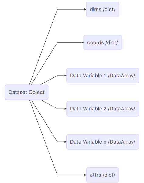
Map of the Dataset object

Now that we’ve completed our survey, we see that a Dataset is a really a kind of container comprised of (actually pointing to) many other objects.

• dims: A dict that maps dimension names (keys) with dimension lengths (values)

• coords: A dict that maps dimension names (keys such as k, j, i) with arrays that label each point in the dimension (values)

• One or more Data Variables that are pointers to DataArray objects

• attrs A dict that maps different attribute names (keys) with the attributes themselves (values).

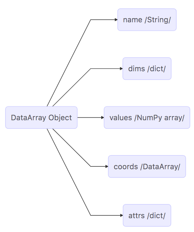
The DataArray Object

It is worth looking at the DataArray object in more detail because DataArrays store the arrays that store the ECCO output. Please see the xarray documentation on the DataArray object for more information.

DataArrays are actually very similar to Datasets. They also contain dimensions, coordinates, and attributes. The two main differences between Datasets and DataArrays is that DataArrays have a name (a string) and an array of values. The values array is a numpy n-dimensional array, an ndarray.

Examining the contents of a DataArray

Let’s examine the contents of one of the coordinates DataArrays found in ds, XC.

ds.XC

<xarray.DataArray 'XC' (tile: 13, j: 90, i: 90)> Size: 421kB
dask.array<open_dataset-XC, shape=(13, 90, 90), dtype=float32, chunksize=(13, 90, 90), chunktype=numpy.ndarray>
Coordinates:
  * i        (i) int32 360B 0 1 2 3 4 5 6 7 8 9 ... 81 82 83 84 85 86 87 88 89
  * j        (j) int32 360B 0 1 2 3 4 5 6 7 8 9 ... 81 82 83 84 85 86 87 88 89
  * tile     (tile) int32 52B 0 1 2 3 4 5 6 7 8 9 10 11 12
    XC       (tile, j, i) float32 421kB dask.array<chunksize=(13, 90, 90), meta=np.ndarray>
    YC       (tile, j, i) float32 421kB dask.array<chunksize=(13, 90, 90), meta=np.ndarray>
Attributes:
    long_name:              longitude of tracer grid cell center
    units:                  degrees_east
    coordinate:             YC XC
    bounds:                 XC_bnds
    comment:                nonuniform grid spacing
    coverage_content_type:  coordinate
    standard_name:          longitude

xarray.DataArray

'XC'

• tile: 13
• j: 90
• i: 90

• dask.array<chunksize=(13, 90, 90), meta=np.ndarray>

  Array Chunk Bytes 411.33 kiB 411.33 kiB Shape (13, 90, 90) (13, 90, 90) Dask graph 1 chunks in 2 graph layers Data type float32 numpy.ndarray

• Coordinates: (5)
  • i
    (i)
    int32
    0 1 2 3 4 5 6 ... 84 85 86 87 88 89

    axis :

    X

    long_name :

    grid index in x for variables at tracer and 'v' locations

    swap_dim :

    XC

    comment :

    In the Arakawa C-grid system, tracer (e.g., THETA) and 'v' variables (e.g., VVEL) have the same x coordinate on the model grid.

    coverage_content_type :

    coordinate

    array([ 0,  1,  2,  3,  4,  5,  6,  7,  8,  9, 10, 11, 12, 13, 14, 15, 16, 17,
           18, 19, 20, 21, 22, 23, 24, 25, 26, 27, 28, 29, 30, 31, 32, 33, 34, 35,
           36, 37, 38, 39, 40, 41, 42, 43, 44, 45, 46, 47, 48, 49, 50, 51, 52, 53,
           54, 55, 56, 57, 58, 59, 60, 61, 62, 63, 64, 65, 66, 67, 68, 69, 70, 71,
           72, 73, 74, 75, 76, 77, 78, 79, 80, 81, 82, 83, 84, 85, 86, 87, 88, 89],
          dtype=int32)

  • j
    (j)
    int32
    0 1 2 3 4 5 6 ... 84 85 86 87 88 89

    axis :

    Y

    long_name :

    grid index in y for variables at tracer and 'u' locations

    swap_dim :

    YC

    comment :

    In the Arakawa C-grid system, tracer (e.g., THETA) and 'u' variables (e.g., UVEL) have the same y coordinate on the model grid.

    coverage_content_type :

    coordinate

    array([ 0,  1,  2,  3,  4,  5,  6,  7,  8,  9, 10, 11, 12, 13, 14, 15, 16, 17,
           18, 19, 20, 21, 22, 23, 24, 25, 26, 27, 28, 29, 30, 31, 32, 33, 34, 35,
           36, 37, 38, 39, 40, 41, 42, 43, 44, 45, 46, 47, 48, 49, 50, 51, 52, 53,
           54, 55, 56, 57, 58, 59, 60, 61, 62, 63, 64, 65, 66, 67, 68, 69, 70, 71,
           72, 73, 74, 75, 76, 77, 78, 79, 80, 81, 82, 83, 84, 85, 86, 87, 88, 89],
          dtype=int32)

  • tile
    (tile)
    int32
    0 1 2 3 4 5 6 7 8 9 10 11 12

    long_name :

    lat-lon-cap tile index

    comment :

    The ECCO V4 horizontal model grid is divided into 13 tiles of 90x90 cells for convenience.

    coverage_content_type :

    coordinate

    array([ 0,  1,  2,  3,  4,  5,  6,  7,  8,  9, 10, 11, 12], dtype=int32)

  • XC
    (tile, j, i)
    float32
    dask.array<chunksize=(13, 90, 90), meta=np.ndarray>

    long_name :

    longitude of tracer grid cell center

    units :

    degrees_east

    coordinate :

    YC XC

    bounds :

    XC_bnds

    comment :

    nonuniform grid spacing

    coverage_content_type :

    coordinate

    standard_name :

    longitude

    Array Chunk Bytes 411.33 kiB 411.33 kiB Shape (13, 90, 90) (13, 90, 90) Dask graph 1 chunks in 2 graph layers Data type float32 numpy.ndarray

  • YC
    (tile, j, i)
    float32
    dask.array<chunksize=(13, 90, 90), meta=np.ndarray>

    long_name :

    latitude of tracer grid cell center

    units :

    degrees_north

    coordinate :

    YC XC

    bounds :

    YC_bnds

    comment :

    nonuniform grid spacing

    coverage_content_type :

    coordinate

    standard_name :

    latitude

    Array Chunk Bytes 411.33 kiB 411.33 kiB Shape (13, 90, 90) (13, 90, 90) Dask graph 1 chunks in 2 graph layers Data type float32 numpy.ndarray

• Indexes: (3)
  • i
    PandasIndex

    PandasIndex(Index([ 0,  1,  2,  3,  4,  5,  6,  7,  8,  9, 10, 11, 12, 13, 14, 15, 16, 17,
           18, 19, 20, 21, 22, 23, 24, 25, 26, 27, 28, 29, 30, 31, 32, 33, 34, 35,
           36, 37, 38, 39, 40, 41, 42, 43, 44, 45, 46, 47, 48, 49, 50, 51, 52, 53,
           54, 55, 56, 57, 58, 59, 60, 61, 62, 63, 64, 65, 66, 67, 68, 69, 70, 71,
           72, 73, 74, 75, 76, 77, 78, 79, 80, 81, 82, 83, 84, 85, 86, 87, 88, 89],
          dtype='int32', name='i'))

  • j
    PandasIndex

    PandasIndex(Index([ 0,  1,  2,  3,  4,  5,  6,  7,  8,  9, 10, 11, 12, 13, 14, 15, 16, 17,
           18, 19, 20, 21, 22, 23, 24, 25, 26, 27, 28, 29, 30, 31, 32, 33, 34, 35,
           36, 37, 38, 39, 40, 41, 42, 43, 44, 45, 46, 47, 48, 49, 50, 51, 52, 53,
           54, 55, 56, 57, 58, 59, 60, 61, 62, 63, 64, 65, 66, 67, 68, 69, 70, 71,
           72, 73, 74, 75, 76, 77, 78, 79, 80, 81, 82, 83, 84, 85, 86, 87, 88, 89],
          dtype='int32', name='j'))

  • tile
    PandasIndex

    PandasIndex(Index([0, 1, 2, 3, 4, 5, 6, 7, 8, 9, 10, 11, 12], dtype='int32', name='tile'))

• Attributes: (7)

  long_name :

  longitude of tracer grid cell center

  units :

  degrees_east

  coordinate :

  YC XC

  bounds :

  XC_bnds

  comment :

  nonuniform grid spacing

  coverage_content_type :

  coordinate

  standard_name :

  longitude

Examining the DataArray

The layout of DataArrays is very similar to those of Datasets. Let’s examine each part of ds.XC, starting from the top.

1. Object type

<xarray.DataArray>

This is indeed a DataArray object from the xarray package.

Note: You can also find the type of an object with the type command: print type(ds.XC)

print (type(ds.XC))

<class 'xarray.core.dataarray.DataArray'>

2. Object Name

XC

The top line shows DataArray name, XC.

3. Dimensions

(tile: 13, j: 90, i: 90)

Unlike THETA, XC does not have time or depth dimensions which makes sense since the longitude of the grid cell centers do not vary with time or depth.

4. The numpy Array

array([[[-111.60647 , -111.303   , -110.94285 , ...,   64.791115,
           64.80521 ,   64.81917 ],
        [-104.8196  , -103.928444, -102.87706 , ...,   64.36745 ,
           64.41012 ,   64.4524  ],
        [ -98.198784,  -96.788055,  -95.14185 , ...,   63.936497,
           64.008224,   64.0793  ],
        ...,

In Dataset objects there are Data variables. In DataArray objects we find numpy arrays. Python prints out a subset of the entire array.

Note: DataArrays store only one array while DataSets can store one or more DataArrays.

We access the numpy array by invoking the .values command on the DataArray.

print(type(ds.XC.values))

<class 'numpy.ndarray'>

The array that is returned is a numpy n-dimensional array:

type(ds.XC.values)

numpy.ndarray

Being a numpy array, one can use all of the numerical operations provided by the numpy module on it.

** Note: ** You may find it useful to learn about the operations that can be made on numpy arrays. Here is a quickstart guide: https://docs.scipy.org/doc/numpy-dev/user/quickstart.html

We’ll learn more about how to access the values of this array in a later tutorial. For now it is sufficient to know how to access the arrays!

4. Coordinates

The dimensional coordinates (with the asterixes) are

Coordinates:
  * j        (j) int32 0 1 2 3 4 5 6 7 8 9 10 ... 80 81 82 83 84 85 86 87 88 89
  * i        (i) int32 0 1 2 3 4 5 6 7 8 9 10 ... 80 81 82 83 84 85 86 87 88 89
  * tile     (tile) int32 0 1 2 3 4 5 6 7 8 9 10 11 12

We find three 1D arrays with coordinate labels for j, i, and tile.

ds.XC.coords

Coordinates:
  * i        (i) int32 360B 0 1 2 3 4 5 6 7 8 9 ... 81 82 83 84 85 86 87 88 89
  * j        (j) int32 360B 0 1 2 3 4 5 6 7 8 9 ... 81 82 83 84 85 86 87 88 89
  * tile     (tile) int32 52B 0 1 2 3 4 5 6 7 8 9 10 11 12
    XC       (tile, j, i) float32 421kB dask.array<chunksize=(13, 90, 90), meta=np.ndarray>
    YC       (tile, j, i) float32 421kB dask.array<chunksize=(13, 90, 90), meta=np.ndarray>

two other important coordinates here are tile and time

print('tile: ')
print(ds.tile.values)
print('time: ')
print(ds.time.values)

tile:
[ 0  1  2  3  4  5  6  7  8  9 10 11 12]
time:
['2010-01-16T12:00:00.000000000' '2010-02-15T00:00:00.000000000'
 '2010-03-16T12:00:00.000000000' '2010-04-16T00:00:00.000000000'
 '2010-05-16T12:00:00.000000000' '2010-06-16T00:00:00.000000000'
 '2010-07-16T12:00:00.000000000' '2010-08-16T12:00:00.000000000'
 '2010-09-16T00:00:00.000000000' '2010-10-16T12:00:00.000000000'
 '2010-11-16T00:00:00.000000000' '2010-12-16T12:00:00.000000000']

The files we loaded contain the monthly-mean potential temperature and salinity fields for each month in 2010. Here the time coordinates are the center of the averaging periods.

5. Attributes

Attributes:
    units:          degrees_east
    long_name:      longitude at center of tracer cell
    standard_name:  longitude_at_c_location
    valid_range:    -180., 180.

The XC variable has a long_name (longitude at center of tracer cell) and units (degrees_east) and other information. This metadata was loaded from the NetCDF file. The entire attribute dictionary is accessed using .attrs.

ds.XC.attrs

{'long_name': 'longitude of tracer grid cell center',
 'units': 'degrees_east',
 'coordinate': 'YC XC',
 'bounds': 'XC_bnds',
 'comment': 'nonuniform grid spacing',
 'coverage_content_type': 'coordinate',
 'standard_name': 'longitude'}

ds.XC.attrs['units']

'degrees_east'

Map of the DataArray Object

The DataArray can be mapped out with the following diagram:

Summary

Now you know the basics of the Dataset and DataArray objects that will store the ECCO v4 model grid parameters and state estimate output variables. Go back and take a look athe grid object that we originally loaded. It should make a lot more sense now!